Thirty three thousand companies will risk fines of 600,000 euros for failing to protect data. The law requires that the files are notified to the English Agency for Data Protection, although only 10% of commercial companies in Jaén (Spain) compliant. Source: Ideal.
Monday, March 31, 2008
Ripper Walmart Black Friday
Index
Topics Index
Section 1: Introduction
Section 2: linear adjustment formulas
Section 3: The least-squares parabola
Section 4: A general matrix method
Section 5: Adjustment to non-linear formulas
Section 6: The ultimate formulas rational
Section 7: The selection of the best model
Section 8: Modeling of interaction effects
Section 9 : Other modeling techniques
Sunday, March 30, 2008
Why Do I Have A Bump Near My
1: Introduction

This work is motivated by the need for accessible practical examples a series of topics that should be a compulsory part of curriculum of any individual who is pursuing an academic career in science and engineering and, unfortunately, not part of the subjects taught in many universities which if mentioned something about it maybe it happens at the end of the introductory courses in the field of statistics, and that if you have time to talk about it after consuming most of the time introducing the student to the theory of probabilities, the hypergeometric distribution the binomial distribution, normal distribution, the t-distribution, analysis of variance over what is scope to do after dealing with these issues, leaving little time to teach the student that perhaps should be the first thing you should learn why this has vast applications in various branches of human knowledge.
start with a very practical question:
If we are not pursuing a degree in Mathematics, what is the reason to spend much of our time to a matter which is essentially part of a branch of mathematics, statistics? What is the reason why we should be motivated to further increase our already heavy burden of study with something like the data set formulas?
To answer this question, we see first that the study of mathematical techniques used to "adjust" data obtained experimentally based formulas preset is indispensable to "endorse" our theoretical scientific models with what is observed in practice all days in the laboratory. Take for example the law of universal gravitation first enunciated by Sir Isaac Newton, which tells us that two bodies of masses M 1 and M 2 attract :

con una fuerza F g que va en razón directa del producto de sus masas y en razón inversa del cuadrado de la distancia d que separa sus centros , lo cual está resumido en la siguiente fórmula:

Este concepto es tan elemental y tan importante, que incluso no se requiere llegar hasta la universidad para ser introducido a él, forma parte de los cursos básicos de ciencias naturales en las escuelas secundaria y preparatoria. Sin usar aún números, comparativamente hablando las consecuencias de ésta fórmula We can summarize the following examples:

In the upper left corner we have two equal masses whose geometric centers are separated by a distance d , which are attracting with a force F . In the second row and in the same column, both masses M are twice the original value, and therefore the force of attraction between these bodies will four times greater, or 4F , since force Attraction is directly proportional to the product of the masses. And in the third row only one of the masses is increased, three times its original value, thus the attraction will be three times higher, rising to 3F. In the right column, the masses are separated at a distance 2d which is twice the original distance, and therefore the force of attraction between them falls not in the middle but a quarter of original value because the attractive force varies inversely with the distance but not the square of the distance separating the masses. And on the third line on the right column the force of attraction between masses increases the Quad to be brought closer to the masses half the original distance. And as we see in the lower right corner, if both masses are increased twice and if the distance between their geometric centers is also increased to twice the force of attraction between them will not change.
far we have been speaking in purely qualitative terms. If we talk in terms quantitative, using numbers , then there is something we need to use the formula given by Newton. We must determine the value of G, the universal gravitational constant . While we can not do that, we will not go very far to use this formula to predict movements of the planets around the sun or the movement of the Moon around the Earth. And this constant G is not something that can be determined theoretically, like it or not we have to go to the lab to perform some kind of experiment with which we can get the value of G , which turns out to be:

experiments in which although it is tempting to immediately get a formula of "best fit" to a series of data, such a formula will do little to reach a conclusion or really important discovery that can be removed with a little cunning in the study of the accumulated data. An example is the following problem (problem 31) taken from chapter 27 (The Electrical Field) of the book "Physics for Engineering and Science Students" by David Halliday and Robert Resnick
PROBLEM: One of his first experiments (1911) Millikan found that, among other charges, appeared at different times as follows, measured at a particular drop:
data in increasing order of magnitude, we can make a graph of them who happens to be the next (this chart and other productions in this work can be seen more clearly or even in some cases expanded with the simple expedient of enlarge):

is important to note that this chart is not an independent variable (whose value would be placed on the horizontal axis) and a dependent variable (whose value would be placed on the vertical axis) as the horizontal axis simply been assigned a different ordinal number to each of the experimental values \u200b\u200blisted, so the first item (1) has a value of 6,563 • 10 -19 , the second data (2) has a value of 8,204 • 10 -19 , and so on.
We can, if we want to obtain a straight line of best fit for these hand-drawn data. But this entirely misses the perspective of the experiment. A chart much more useful than the dot plot shown above is the following graph of the data known as graphical ladder or step graphical :

carefully inspecting the graph of this data, We realize that there are "steps" which seems to be the same height of a datum to the next. The difference between observations 1 and 2, for example, seems to be the same as the difference between observations 6 and 7. And those "gaps" where it is not, seems to be height twice the height other steps. If the height of a step to the next did not have this similarity with any of the remaining observations, we may conclude that the differences are completely random. But this is not what is happening and the steps seem to have heights equal to or double equal. These data are revealing something important, that electric charge is quantized , the electric charge reported here does not vary much from 0.7, 1.4 or 2.5, but integral multiples of one or two goals. The data we are confirming the existence of the electron , the smallest electric charge is no longer possible subdivided by physical or chemical means at our disposal. Among the data on which the "jump" from one step to another is double from that in other steps, we can conclude that data are "missing" and that an additional amount of experiments, it should be possible to find experimental values \u200b\u200bbetween those jumps "doubles" that posts in the graph, we must produce a staircase with steps of similar height could be called "basic." By way of example, the reported value of 11.50 • 10 -19 coulombs and 8,204 • 10 -19 coulombs must have an intermediate value of about 9,582 • 10 -19 coulombs with an additional recabación laboratory data should be possible to detect sooner or later.
We can estimate the magnitude of the electric charge as we now know as the electron by first obtaining the differences between the data representing a unit jump by averaging them, and after that the differences between the data representing a jump "double" also getting the same average and dividing the result of the latter two, summing and averaging the two sets of values \u200b\u200band for a final result:
Set 1 (Jump Unit):
And the average of the second data set is:
that it be divided into two:
Since there are so many data ( 4 data) in the first set and in the second set, we can give the same "simple weight" to each of the averages obtained by adding the average first to second average and dividing the result by two (of not being so, both teams have had a different number of observations, we have to give a "significant factor" arithmetic each set to give each contribution according to their relative importance):
As a postscript to this problem, which is added later experiments conducted with greater precision and minimizing sources of error with a seeking of a large number of data (which helps to gradually reduce the random error due to causes beyond the control of the experimenter) leads to a more accurate value of 1.60 • 10 -19 coulombs for the electron charge, which is the accepted value today.


This work is motivated by the need for accessible practical examples a series of topics that should be a compulsory part of curriculum of any individual who is pursuing an academic career in science and engineering and, unfortunately, not part of the subjects taught in many universities which if mentioned something about it maybe it happens at the end of the introductory courses in the field of statistics, and that if you have time to talk about it after consuming most of the time introducing the student to the theory of probabilities, the hypergeometric distribution the binomial distribution, normal distribution, the t-distribution, analysis of variance over what is scope to do after dealing with these issues, leaving little time to teach the student that perhaps should be the first thing you should learn why this has vast applications in various branches of human knowledge.
start with a very practical question:
If we are not pursuing a degree in Mathematics, what is the reason to spend much of our time to a matter which is essentially part of a branch of mathematics, statistics? What is the reason why we should be motivated to further increase our already heavy burden of study with something like the data set formulas?
To answer this question, we see first that the study of mathematical techniques used to "adjust" data obtained experimentally based formulas preset is indispensable to "endorse" our theoretical scientific models with what is observed in practice all days in the laboratory. Take for example the law of universal gravitation first enunciated by Sir Isaac Newton, which tells us that two bodies of masses M 1 and M 2 attract :

con una fuerza F g que va en razón directa del producto de sus masas y en razón inversa del cuadrado de la distancia d que separa sus centros , lo cual está resumido en la siguiente fórmula:

Este concepto es tan elemental y tan importante, que incluso no se requiere llegar hasta la universidad para ser introducido a él, forma parte de los cursos básicos de ciencias naturales en las escuelas secundaria y preparatoria. Sin usar aún números, comparativamente hablando las consecuencias de ésta fórmula We can summarize the following examples:

In the upper left corner we have two equal masses whose geometric centers are separated by a distance d , which are attracting with a force F . In the second row and in the same column, both masses M are twice the original value, and therefore the force of attraction between these bodies will four times greater, or 4F , since force Attraction is directly proportional to the product of the masses. And in the third row only one of the masses is increased, three times its original value, thus the attraction will be three times higher, rising to 3F. In the right column, the masses are separated at a distance 2d which is twice the original distance, and therefore the force of attraction between them falls not in the middle but a quarter of original value because the attractive force varies inversely with the distance but not the square of the distance separating the masses. And on the third line on the right column the force of attraction between masses increases the Quad to be brought closer to the masses half the original distance. And as we see in the lower right corner, if both masses are increased twice and if the distance between their geometric centers is also increased to twice the force of attraction between them will not change.
far we have been speaking in purely qualitative terms. If we talk in terms quantitative, using numbers , then there is something we need to use the formula given by Newton. We must determine the value of G, the universal gravitational constant . While we can not do that, we will not go very far to use this formula to predict movements of the planets around the sun or the movement of the Moon around the Earth. And this constant G is not something that can be determined theoretically, like it or not we have to go to the lab to perform some kind of experiment with which we can get the value of G , which turns out to be:

But the determination of this constant mark just the beginning of our work. We assume that this formula was given under certain laboratory conditions in which there were two masses separated by a distance known as accurately as possible. The exponent 10 -11 that appears in the numerical value the constant G tells us in a way that the effect to be measured is extremely small, which is expected, because two smaller masses the size of a marble used for the experiment will be attracted to a very weak force barely detectable almost . The existence of a force of attraction between two small masses can be confirmed in an experiment of medium complexity, this does not present major challenges. But the measure G constant and not only to find that two bodies attract represents serious difficulties. The first to evaluate the constant G was Cavendish laboratory, who used a device that was essentially a torsion balance by implementing the next schmo:

Although at first glance one thinks of the possibility of increasing all bodies used in the experiment to make the effect more intense attraction between them, no such thing can lead to out moving masses (red) without bursting the thin thread which hangs these weights. You can, however, increase the mass of blue, and this was precisely what he did Cavendish. Note that there are only two masses being attracted but two pairs allying mass, which increases the effect on the torsion balance. Either way, the enormous difficulties in obtaining a numerical value G reliable under this experiment will not increase our confidence in the value of G thus obtained.
However, a value of G obtained under these conditions and put in the formula does not guarantee that the formula will work as predicted by Newton for other conditions that are very different from the conditions used in the laboratory, which involved masses much greater distances. This formula is not the only one who can give us an attractive force between two masses decreases with increasing distance between the geometric centers of the masses. We can formulate a law that says: "Two bodies attract because direct product of their masses and inversely as the distance that separates them. "Note the absence of the term" square of the distance separating them. And we can make both formulas coincide numerically for some distance apart, but the variation in the strength of attraction given by the two formulas, it will become more and more evident as the masses are being brought closer or separated more and more. As both formulas, mathematically different, are not equally valid to describe the same phenomenon, one has to be discarded with the help of experimentally obtained data . Again we have to go to the lab. The confirmation of Newton's law is valid we get if we can measure the force of attraction for various distances by a graph of the results. For a variation inversely proportional to the square of the distance, the graph should be as follows:

one way or another, are laboratory experiments that help us to confirm or rule out any theory like this. And in experiments difficult by their very nature, which introduces a statistical random error that we can introduce experimental variation in each reading we take, we are almost obliged to collect the maximum amount of data to increase the reliability of the results, in which case the problem will be trying to draw any conclusion from the mass of data collected, because you can not expect all or perhaps none of the data will "fall" smoothly and accurately on a continuous curve. This forces us to try to find somehow the mathematical expression for a smooth, continuous curve, among many other possible ones, that best fits the experimental data.
case we have spoken this is the typical case in that before carrying out measurements in the laboratory and there is a theoretical model -a formula - waiting to be confirmed experimentally by measurements or observations made after the formula was obtained. But many other cases in which although experimental data, despite the unavoidable sources of variation and measurement errors seem to follow any law that can be adjusted to a theoretical model, such a formula does not exist, either because they have not found or perhaps because it is too complex to be stated in a few lines. In such cases the best we can do is carry out the fit of the data obtained experimentally to a empirical formula, a formula selected from many to be the one that best fits the data. The most notorious example of this today has to do with the alleged global warming on Earth, confirmed independently by several experimental data collected over several decades in many places around the Earth. Still no exact formula or even an empirical formula that allows us to predict the Earth's temperatures will be in later years if things continue as usual. All we have are graphs in which, broadly speaking, one can see a tendency towards a gradual increase in temperature, inferred from the data trend ( trend data), and even some of these data are cause controversial, such as temperature data registered in Punta Arenas, Chile, between 1888 and 2001:

Often, when carrying out the plotting of the data (the most important step prior to the selection of the mathematical model which will try to "adjust" the data) since before attempting to carry out the adjustment data to a formula we can detect the presence of an abnormality in the same due to an unexpected source of error that has nothing to do with the error of a statistical nature, as shown in the following graph of the temperatures of lakes in Detroit:

Note
carefully on this chart that there are two points that were not linked with lines for researchers to highlight the presence of a serious anomaly in the data. These are the points representing the end of 1999 and early 2000. As we begin 2000, the data show a "jump" disproportionate to the data prior history. Although we try to force all data are grouped under a certain trend predicted by an empirical formula, an anomaly as seen in this graph we practically cries out for explanation before being buried in such empirical formula. A review of the data revealed that, indeed, the "jump" disproportionate had to do with a phenomenon that was already expected at that time was going to happen with some computer systems are not prepared for the consequences of the change of digits in the date 1999 to 2000, then dubbed as the Y2K phenomenon (an acronym for the phrase " Y ear 2000" where k symbolizes thousand). The discovery of this effect gave rise to an exchange of explanations documented in places like the following:
http://www.climateaudit.org/?p=1854
http://www.climateaudit.org/?p=1868
This exchange for clarification led to the same U.S. space agency NASA to correct their own data, taking into account the effect Y2k, and corrected data displayed on the following site:
http://data.giss.nasa.gov/gistemp/graphs/
Fig.D.txt
The examples we have seen have been instances in which the experimental data despite variations in the same setting allows them to approximate a mathematical formula or even allow the detection of some error in gathering them. But there are many other occasions in which to carry out the data to plot the presence of a trend is not at all obvious, as shown in the following sample data collected on the frequency of sunspots (which may have some effect on global warming of the Earth):

In the graph of the data has been superimposed a red line under a statistical mathematical criterion represents the line of best fit to the data. But in this case this line is clearly an obvious decline, including online almost seems to be a horizontal line. If you delete line, the data seem so scattered that have chosen a straight line to try to "bundle" the trend of data seems rather an act of faith than scientific objectivity. It may be no reason to expect a statistically significant change on the frequency of sunspots over the course of several centuries or even several thousand years, given the enormous complexity of the nuclear processes that keep the Sun in constant activity. This last example demonstrates the enormous difficulties that face any researcher trying to analyze a set of experimental data on which there is any theoretical model.
The data set formulas is of vital importance always bear in mind the law of cause and effect . In the case of the law of universal gravitation, as set forth by an exact formula, assuming the masses of two bodies as unchanged, then a variation of the distance between the masses will have a direct effect on the strength of gravitational attraction is between them. A series of experimental data on a chart positions will confirm this. And even in cases where there is an exact model, we can (or rather, we need to) make a cause-effect relationship for a model of two variables can have some meaning. Such is the case when performing measurements of stature between students of different grades of elementary school. In this case, the average heights for each grade students will be different, it will increase as increasing the grade, for the simple fact that students at this age are growing in stature every year. In short, the higher the grade, the higher the average height of students who expect to find in a group. This is a cause-effect relationship. In contrast, if we find a direct relationship between the temperature of a city for one day of the year and the number of pets that people have in their homes, most likely will not find any relationship and come out empty handed because there is no reason to expect that the average number of pets per household (case) may have some influence on the temperature (effect), and if so, this effect would be negligible by mathematically smallness.
we have seen cases involve situations based on natural phenomena which we can carry out measurements in the laboratory or outside the laboratory using something as simple as a thermometer or as an amateur telescope. But there are many other cases in which it is not necessary to conduct measurements, because more than getting data in the lab what is needed is a mathematical model that allows us to make a projection or prediction with data already on hand, as data from a census or a survey. An example is the expected growth of Mexico's annual population. The national population census is to be in charge of obtaining figures on the population of Mexico, so that to try to make a prediction on the expected population growth in future years all we have to do is go to National Institute of Statistics, Geography and Informatics (INEGI) for the results of previous censuses. It is assumed that in these census figures are not exact, there is no reason to expect such a thing, given the enormous number of variables that have to deal with workers who must carry out the census and the changing day to day can affect the "reality" of the census. Even assuming that the census could be carried out exactly, we would be another problem. If we plot the population ratios of 5 years (for example), there would be no problem in making future predictions based on past data if the data when plotted fall all in a "straight line". The problem is that, when plotted almost never fall on a straight line, usually grouped around what appears to be a curve . Here we try to "adjust" the data to a Various formulas and use the one that best approximates all the data you already have, for which we need a mathematical-statistical approach that is less subjective as possible. It is precisely for this so we require the principles to be discussed here.
The data adjustment formulas, there are cases in which it is not necessary to go into detailed mathematical calculations for the simple reason that for such cases have been obtained and formulas that only require the calculation of simple things such as the arithmetic mean (often designated as μ, the Greek letter mu equivalent of the Latin letter "m", so on average arithmetic) data and standard deviation σ (the Greek letter sigma , the equivalent of the Latin letter "s" so the "standard") of them. We are referring to adjust the data to a Gaussian curve . One such adjustment is applied to situations where instead of having a dependent variable and whose values \u200b\u200bdepend on the values \u200b\u200bthat can make an independent variable X on which perhaps we can exercise some control data set in which what matters is the frequency with which data are collected are located within certain ranges. An example would be grades in certain subjects in a group number of 160 students whose scores show a distribution as follows:

The way in which data are presented, we must make a slight modification in our calculations to obtain the average arithmetic them, using as the representative value of each interval the average value between the minimum and maximum of each interval. Thus, the representative value of the interval between a score of 4.5 and 5.0 is 4.75, the representative value in the range between 5.0 and 5.5 is 5.25, and so on. Each of these values \u200b\u200brepresentative of each interval we have to give weight "fair" that belongs in the calculation of the mean multiplied by the frequency with which it occurs. Thus, the value 4.75 is multiplied by 4 since that is the frequency with which it occurs, and the value 5.25 is multiplied by 7 since that is the frequency with which it occurs, and so on. Thus, the arithmetic mean of the population of 150 students will:
Having obtained the average arithmetic X , the next step would be to obtain the dispersion of these data with respect to the arithmetic average, through a calculation and variance σ ² in which we average the sum of the squares of the differences d i of each data with respect to the arithmetic mean for the variance σ ² population data:
with which we can obtain the standard deviation σ population data (also known as the root mean square deviation-of-range data to the arithmetic mean) with the simple operation of taking the square root of variance: σ
worth noting that the standard deviation σ evaluated for a sample taken at random from a population has a slightly different definition of the standard deviation σ evaluated on all data the total of the population. The standard deviation σ sample of a population is obtained by replacing the term N in the denominator N-1, because the words of the "purists" value obtained is a better estimate of the standard deviation of the population from which the sample was taken. However, for sufficiently large sample (N greater than 30), there is little difference between the two estimates of σ . Anyway, when you want to get a "best estimate" can always be obtained by multiplying the standard deviation we have defined √ N/N-1 . It is important to bear in mind that σ is a somewhat arbitrary measure of data dispersion, is something that we have defined ourselves, and we use N-1 instead of N actually denominator is not an absolute. However, it is a universally accepted convention, perhaps among other things (besides the theoretical reasons cited by purists) and the fact that to calculate a dispersion of information is required at least two data, which is implicitly recognized by using N-1 in the denominator since this way is not possible to give N worth one without falling into a division by zero, the definition used N-1 removed from the scene any possible interpretation of σ with only one value. And another important reason has more to do with the reasons given by the purists is that the use of N-1 in the denominator has to do with something called the degrees of freedom in the analysis of variance ANOVA known as (Analysis of Variance ) used in the design of experiments (though that's get out a bit of subject we are discussing this document).
In descriptive statistics, which is carried out taking all values \u200b\u200bof a population of data and not taking a sample of that population, the most important of the graph of the relative frequencies of the data or histogram is the "area under the curve" rather than the formula of the curve to be pass by "height" of each data, the curve being used to find the mathematical probability of having a group of students from a range of scores, for example between 7.5 and 9.0, a mathematical probability value always lies between zero and unity. This is what is traditionally taught in textbooks.
However, before applying the statistical tables to carry out some probabilistic analysis of the area under the curve ", it is interesting how well the data fit a continuous curve can be drawn connecting the heights of the histogram. The formula that best describes a set of data which have been shown in the example is one that gives rise to the Gaussian curve . Then, to the following formula "Gaussian"

have the graph of the continuous curve drawn by this formula:

As can be seen, the curve indeed has the form of a bell, which derives a name with cuales es conocida.
Se puede demostrar, recurriendo a un criterio matemático conocido como el método de los mínimos cuadrados, que una fórmula general que modela una curva Gaussiana a un conjunto dado de datos con la apariencia de una "campana" es la siguiente:

Y resulta que µ es precisamente la media aritmética de la población de datos designada también como X , mientras que σ² es la varianza presentada por la población de datos. Esto signica que, para modelar una curva a un conjunto de datos como el que hemos estado manejando en el ejemplo, basta con calcular the mean and variance of the data, and put this information directly to the Gaussian formula, which will curve "best fit" (under the criterion of least squares) to the data. Parameter evaluation A no problem, since the curve must reach (but not exceeding) to a height of 34 (the number of students who represent the greater frequency with respect to other ranks of skills) so that the formula of the curve fitted to the data example is the following:

The graph of this Gaussian curve, superimposed on the graph bar that contains discrete data from which it was generated, is as follows:
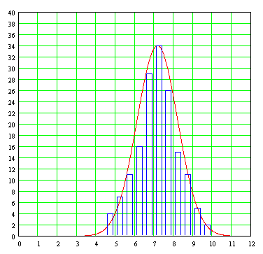
We can see that the fit is reasonably good, considering the fact that in real life or experimental data never observed exactly fit the ideal Gaussian curve.
One thing which we must deal from the start, which almost never sufficiently clarified and explained well in the classroom is the fact that the general Gaussian formula not only allows positive values \u200b\u200bof X but also even allows values negative , which have no interpretation in the real world in cases like the one just see (on a grading system for students as we are assuming, any qualification can only vary from zero to ten minimum qualification as highest). In principle, X can range from X to X =- ∞ = + ∞. In many cases this is no problem, since the curve is rapidly approaching zero before X goes down to zero taking negative values, as in our example where the arithmetic is sufficiently far from X = 0 and dispersion of data is small enough to consider negative values \u200b\u200bof X as irrelevant, although the formula allows. But in cases in which the arithmetic mean X is too close to X = 0 and the data show a large dispersion, there is always the possibility that a complete end of the curve dropping the "other side" in the zone for which X takes negative values . If this happens, it could even force us to abandon the Gaussian model and other alternatives that will certainly be more unpleasant to handle from a mathematical point of view.
has provided a procedure to obtain the formula of a curve to connect the height of each bar of a histogram data showing the shape of the "bell", but it is important to clarify that individual points curve without real meaning, which is equivalent to say that a point as X = 7.8 for which the value of Y is equal to 28,595 is not something we should mean absolutely nothing, since it is the region under curve which makes sense, since the curve was generated from histogram bars that change from one interval to another. However, what we have done here is justified for comparative purposes because, before applying our notions of statistical data set using the Gaussian distribution about whether they want to make sure the data we analyze are shaped like a bell, because if data seem to follow a linear trend ever upward or if instead of a bell we have two bells (the latter occurs when data is accumulated from two different sources), would be wrong to try to force such data on a Gaussian distribution. It is important to add that we have seen the curve is not symmetrical distribution studied in statistical texts, as so we must normalize formula so that not only the arithmetic mean is shifted to the left the diagram to have a zero value to both sides being symmetrical with respect to X = o, but also the area under the curve has the value unity, this in order to give a performance curve probability as applied to non-descriptive statistics but inferential statistics in which a random sample trying to figure out the behavior of the data from a general population. In this normalization process derives its name from the curve as normal curve.
Before trying to invest time and effort to set a formula empirical data before doing any arithmetic, it is important to an early graphical data, as this is the first thing that must guide us in selecting the mathematical model to be used for modeling. In the case of distributions frequency as we've seen, which are represented by histograms, if doing a graph of the data we get something like the following:

then if we can "force" the data to fall within a formula modeled on a continuous independent variable whose stroke is "fit" to the heights of the bars of the histograms, obtaining in this last example a setting like this (this adjustment is carried out simply by adding the expressions for two Gaussian curves with means other than by changing individual variances and amplitudes of each curve to the score):

this setting is a setting meaningless, since a chart like this, known as graphical bimodal, which has two "caps" peaks, is telling us that instead of having a population of data the same source we have is two populations of different origins data, data that came tucked into a single "package" at the hands of the analyst. This is when the analyst is almost forced to go to the "field" to see how and where data were collected. It is possible that the data represent the lengths of certain beams which were produced by two different machines. It is also possible These data have originated in an experiment in which he was testing the effect of a new type of fertilizer on yield of some crops and the fertilizer was being supplied to experimental plots for two different people in two different places, in which case there something that is causing a significant difference in the performance of the fertilizer and the effect it may have the fertilizer itself, either that both persons have been supplying different quantities of the same fertilizer, or the characteristics of different areas have caused Gaussian distribution altered the performance of each type of fertilizer.
For the continuous curve "double hump" shown above, this curve was drawn by the following formula score obtained by adding two Gaussian curves and setting the "top" of each curve to match the approximate-manipulating the arithmetic mean μ at each end-caps with each of the two top bars, modifying also the variance σ in each term for "open" or "close" the width of each fitted curve will:

Then we separated individual plots (not added) to each of the Gaussian curves shown in the formula, showing a probable range of data from two distinct populations of which came from the scrambled data.
In this example, it was easy to just view the histogram, the bar graph data-the presence of two Gaussian curves instead of one, thanks to the arithmetic mean of each curve (5.7 and 10.4) are separated by a margin of almost two to one. But we will not always so lucky, and there will be cases in which the arithmetic will be so close to each other that will be somewhat difficult for the analyst to decide if it considers all data as one or try to find two different curves, as would occur with a graph whose curve joining the heights of the bars would look like this:

is in cases like these in which the analyst must draw on all her wit and all his experience to decide if he tries to find two discernible groups of data in the data set at hand, or if it is not worth for the presence of two distinct populations riots in one, opting to perform modeling based on a single Gaussian formula.
Discovering the influence of unknown factors that may affect the performance of something as a fertilizer is just one of the primary objectives the design of experiments . In the design of experiments are not interested in carrying out a modeling of the data to a formula, that comes after it has been established unequivocally how many and what are the factors that can affect performance or response to something. Once passed this stage, we can collect data to carry out the adjustment of data to a formula. In the case of a bimodal distribution, instead of trying to set a formula to describe all data with a single distribution as we have seen, is much better to try to separate the data from the two different populations that are causing the "double hump camel ", a fact that can analyze two data sets separately with the assurance that for each data set we obtain a Gaussian distribution with a single hump. It can be seen from this that the formulas data modeling is a continuous cycle experimentation, analysis and interpretation of results, followed by a new cycle of experimentation and analysis and interpretation of new results to be improving a process or could go better describing the data being collected in a laboratory or field. The data modeling formula goes hand in hand with the procedures for the collection of the same.
PROBLEM : experimentally in the laboratory is the boiling point for some organic compounds known as alkanes (chemical formula C n H 2n +2 \u200b\u200b ) has the following values \u200b\u200bin degrees Celsius:
Methane (1 carbon atom): -161.7
ethane (2 carbons): -88.6
propane (3 carbon atoms): -42.1
butane (4 carbons): -0.5
pentane (5 carbon atoms): 36.1
hexane (6 carbon atoms): 68.7
heptane (7 carbons): 98.4
octane (8 carbon atoms): 125.7
Nonane (9 carbon atoms): 150.8
Dean (10 carbon atoms): 174.0
Make a graph of the data. Does it show any tendency the boiling point of these organic compounds according to the number of carbon atoms that have each compound?
The graph of discrete data is as follows:

The graph we can see that the data seem to accommodate a super smooth continuous curve, following the cause-effect, which we suggests that behind this data is a natural law waiting to be discovered by us. Since the data do not follow a straight line, the relationship between them is not a linear relationship, is a non-linear relationship , and do not expect that the mathematical formula that is behind this curve is that of a line straight. In the absence of a theoretical model that allows us to have the exact formula, the graph arising from this data set is an excellent example of the places where we can try to adjust the data to an empirical formula, the better the data fit , the better we will suggest the nature of natural laws operating behind this phenomenon.

Although at first glance one thinks of the possibility of increasing all bodies used in the experiment to make the effect more intense attraction between them, no such thing can lead to out moving masses (red) without bursting the thin thread which hangs these weights. You can, however, increase the mass of blue, and this was precisely what he did Cavendish. Note that there are only two masses being attracted but two pairs allying mass, which increases the effect on the torsion balance. Either way, the enormous difficulties in obtaining a numerical value G reliable under this experiment will not increase our confidence in the value of G thus obtained.
However, a value of G obtained under these conditions and put in the formula does not guarantee that the formula will work as predicted by Newton for other conditions that are very different from the conditions used in the laboratory, which involved masses much greater distances. This formula is not the only one who can give us an attractive force between two masses decreases with increasing distance between the geometric centers of the masses. We can formulate a law that says: "Two bodies attract because direct product of their masses and inversely as the distance that separates them. "Note the absence of the term" square of the distance separating them. And we can make both formulas coincide numerically for some distance apart, but the variation in the strength of attraction given by the two formulas, it will become more and more evident as the masses are being brought closer or separated more and more. As both formulas, mathematically different, are not equally valid to describe the same phenomenon, one has to be discarded with the help of experimentally obtained data . Again we have to go to the lab. The confirmation of Newton's law is valid we get if we can measure the force of attraction for various distances by a graph of the results. For a variation inversely proportional to the square of the distance, the graph should be as follows:

one way or another, are laboratory experiments that help us to confirm or rule out any theory like this. And in experiments difficult by their very nature, which introduces a statistical random error that we can introduce experimental variation in each reading we take, we are almost obliged to collect the maximum amount of data to increase the reliability of the results, in which case the problem will be trying to draw any conclusion from the mass of data collected, because you can not expect all or perhaps none of the data will "fall" smoothly and accurately on a continuous curve. This forces us to try to find somehow the mathematical expression for a smooth, continuous curve, among many other possible ones, that best fits the experimental data.
case we have spoken this is the typical case in that before carrying out measurements in the laboratory and there is a theoretical model -a formula - waiting to be confirmed experimentally by measurements or observations made after the formula was obtained. But many other cases in which although experimental data, despite the unavoidable sources of variation and measurement errors seem to follow any law that can be adjusted to a theoretical model, such a formula does not exist, either because they have not found or perhaps because it is too complex to be stated in a few lines. In such cases the best we can do is carry out the fit of the data obtained experimentally to a empirical formula, a formula selected from many to be the one that best fits the data. The most notorious example of this today has to do with the alleged global warming on Earth, confirmed independently by several experimental data collected over several decades in many places around the Earth. Still no exact formula or even an empirical formula that allows us to predict the Earth's temperatures will be in later years if things continue as usual. All we have are graphs in which, broadly speaking, one can see a tendency towards a gradual increase in temperature, inferred from the data trend ( trend data), and even some of these data are cause controversial, such as temperature data registered in Punta Arenas, Chile, between 1888 and 2001:

According to the graph of this data which is set in a straight line of red that, mathematically speaking, represents the trend Data averaged over time, the temperature in that part of the world has been rising for over a century, but instead has been declining by a cumulative average of 0.6 degrees Celsius, contrary to the measurements have been carried out in other parts of the world. We do not know exactly why that happens there is different from that observed in other parts of world. Possibly there are interactions with sea temperatures, with the climatic conditions in that region of the planet, or even up to the rotation of the Earth, which are influenced to cause a fall rather than a rise in temperature observed at Punta Arenas. Anyway, despite ups and downs of the data, with such data is possible to obtain the straight line of red-superimposed on the data, which mathematically speaking is "fit" better than other lines to the average mobile data accumulated . Trends continue, this straight line allows us to estimate, between high and low that they occur in the data in subsequent years, average temperatures will short term in Punta Arenas in the years ahead. On these data, the line of best fit ( best fit) is a completely empirical formula for which there is as yet no theoretical model to support it. And just as there are many in this formula which is a mathematical model to simplify something that is being observed or measured.
Often, when carrying out the plotting of the data (the most important step prior to the selection of the mathematical model which will try to "adjust" the data) since before attempting to carry out the adjustment data to a formula we can detect the presence of an abnormality in the same due to an unexpected source of error that has nothing to do with the error of a statistical nature, as shown in the following graph of the temperatures of lakes in Detroit:

Note
carefully on this chart that there are two points that were not linked with lines for researchers to highlight the presence of a serious anomaly in the data. These are the points representing the end of 1999 and early 2000. As we begin 2000, the data show a "jump" disproportionate to the data prior history. Although we try to force all data are grouped under a certain trend predicted by an empirical formula, an anomaly as seen in this graph we practically cries out for explanation before being buried in such empirical formula. A review of the data revealed that, indeed, the "jump" disproportionate had to do with a phenomenon that was already expected at that time was going to happen with some computer systems are not prepared for the consequences of the change of digits in the date 1999 to 2000, then dubbed as the Y2K phenomenon (an acronym for the phrase " Y ear 2000" where k symbolizes thousand). The discovery of this effect gave rise to an exchange of explanations documented in places like the following:
http://www.climateaudit.org/?p=1854
http://www.climateaudit.org/?p=1868
This exchange for clarification led to the same U.S. space agency NASA to correct their own data, taking into account the effect Y2k, and corrected data displayed on the following site:
http://data.giss.nasa.gov/gistemp/graphs/
Fig.D.txt
The examples we have seen have been instances in which the experimental data despite variations in the same setting allows them to approximate a mathematical formula or even allow the detection of some error in gathering them. But there are many other occasions in which to carry out the data to plot the presence of a trend is not at all obvious, as shown in the following sample data collected on the frequency of sunspots (which may have some effect on global warming of the Earth):

In the graph of the data has been superimposed a red line under a statistical mathematical criterion represents the line of best fit to the data. But in this case this line is clearly an obvious decline, including online almost seems to be a horizontal line. If you delete line, the data seem so scattered that have chosen a straight line to try to "bundle" the trend of data seems rather an act of faith than scientific objectivity. It may be no reason to expect a statistically significant change on the frequency of sunspots over the course of several centuries or even several thousand years, given the enormous complexity of the nuclear processes that keep the Sun in constant activity. This last example demonstrates the enormous difficulties that face any researcher trying to analyze a set of experimental data on which there is any theoretical model.
The data set formulas is of vital importance always bear in mind the law of cause and effect . In the case of the law of universal gravitation, as set forth by an exact formula, assuming the masses of two bodies as unchanged, then a variation of the distance between the masses will have a direct effect on the strength of gravitational attraction is between them. A series of experimental data on a chart positions will confirm this. And even in cases where there is an exact model, we can (or rather, we need to) make a cause-effect relationship for a model of two variables can have some meaning. Such is the case when performing measurements of stature between students of different grades of elementary school. In this case, the average heights for each grade students will be different, it will increase as increasing the grade, for the simple fact that students at this age are growing in stature every year. In short, the higher the grade, the higher the average height of students who expect to find in a group. This is a cause-effect relationship. In contrast, if we find a direct relationship between the temperature of a city for one day of the year and the number of pets that people have in their homes, most likely will not find any relationship and come out empty handed because there is no reason to expect that the average number of pets per household (case) may have some influence on the temperature (effect), and if so, this effect would be negligible by mathematically smallness.
we have seen cases involve situations based on natural phenomena which we can carry out measurements in the laboratory or outside the laboratory using something as simple as a thermometer or as an amateur telescope. But there are many other cases in which it is not necessary to conduct measurements, because more than getting data in the lab what is needed is a mathematical model that allows us to make a projection or prediction with data already on hand, as data from a census or a survey. An example is the expected growth of Mexico's annual population. The national population census is to be in charge of obtaining figures on the population of Mexico, so that to try to make a prediction on the expected population growth in future years all we have to do is go to National Institute of Statistics, Geography and Informatics (INEGI) for the results of previous censuses. It is assumed that in these census figures are not exact, there is no reason to expect such a thing, given the enormous number of variables that have to deal with workers who must carry out the census and the changing day to day can affect the "reality" of the census. Even assuming that the census could be carried out exactly, we would be another problem. If we plot the population ratios of 5 years (for example), there would be no problem in making future predictions based on past data if the data when plotted fall all in a "straight line". The problem is that, when plotted almost never fall on a straight line, usually grouped around what appears to be a curve . Here we try to "adjust" the data to a Various formulas and use the one that best approximates all the data you already have, for which we need a mathematical-statistical approach that is less subjective as possible. It is precisely for this so we require the principles to be discussed here.
The data adjustment formulas, there are cases in which it is not necessary to go into detailed mathematical calculations for the simple reason that for such cases have been obtained and formulas that only require the calculation of simple things such as the arithmetic mean (often designated as μ, the Greek letter mu equivalent of the Latin letter "m", so on average arithmetic) data and standard deviation σ (the Greek letter sigma , the equivalent of the Latin letter "s" so the "standard") of them. We are referring to adjust the data to a Gaussian curve . One such adjustment is applied to situations where instead of having a dependent variable and whose values \u200b\u200bdepend on the values \u200b\u200bthat can make an independent variable X on which perhaps we can exercise some control data set in which what matters is the frequency with which data are collected are located within certain ranges. An example would be grades in certain subjects in a group number of 160 students whose scores show a distribution as follows:
Between 4.5 and 5.0: 4 studentsThis type of distribution, when plotted, statistically show a tendency to reach a peak in a curve that resembles a bell. The first calculation that we made on such data is the arithmetic average or arithmetic mean defined as
Between 5.0 and 5.5: 7 students
Between 5.5 and 6.0: 11 students
Between 6.0 and 6.5: 16 students
Between 6.5 and 7.0: 29 students
Between 7.0 and 7.5: 34 students
Between 7.5 and 8.0: 26 students
Between 8.0 and 8.5: 15 students
Between 8.5 and 9.0: 11 students
Between 9.0 and 9.5: 5 students
Between 9.5 and 10.0: 2 students

The way in which data are presented, we must make a slight modification in our calculations to obtain the average arithmetic them, using as the representative value of each interval the average value between the minimum and maximum of each interval. Thus, the representative value of the interval between a score of 4.5 and 5.0 is 4.75, the representative value in the range between 5.0 and 5.5 is 5.25, and so on. Each of these values \u200b\u200brepresentative of each interval we have to give weight "fair" that belongs in the calculation of the mean multiplied by the frequency with which it occurs. Thus, the value 4.75 is multiplied by 4 since that is the frequency with which it occurs, and the value 5.25 is multiplied by 7 since that is the frequency with which it occurs, and so on. Thus, the arithmetic mean of the population of 150 students will:
X = [(4) (4.75) + (7) (5.25) + (11) (5.75) +. .. (9.75) (2)] / 160
X = 7,178
X = 7,178
Having obtained the average arithmetic X , the next step would be to obtain the dispersion of these data with respect to the arithmetic average, through a calculation and variance σ ² in which we average the sum of the squares of the differences d i of each data with respect to the arithmetic mean for the variance σ ² population data:
Σd ² = 4 ∙ (4.75-7.178) ² + 7 (5.25-7.178) ² + ... + 2 ∙ (2-7178) ²
178,923
Σd ² = σ ² =
Σd ² / N = 1,118
178,923
Σd ² = σ ² =
Σd ² / N = 1,118
with which we can obtain the standard deviation σ population data (also known as the root mean square deviation-of-range data to the arithmetic mean) with the simple operation of taking the square root of variance: σ
= √ 1118 = 1057
worth noting that the standard deviation σ evaluated for a sample taken at random from a population has a slightly different definition of the standard deviation σ evaluated on all data the total of the population. The standard deviation σ sample of a population is obtained by replacing the term N in the denominator N-1, because the words of the "purists" value obtained is a better estimate of the standard deviation of the population from which the sample was taken. However, for sufficiently large sample (N greater than 30), there is little difference between the two estimates of σ . Anyway, when you want to get a "best estimate" can always be obtained by multiplying the standard deviation we have defined √ N/N-1 . It is important to bear in mind that σ is a somewhat arbitrary measure of data dispersion, is something that we have defined ourselves, and we use N-1 instead of N actually denominator is not an absolute. However, it is a universally accepted convention, perhaps among other things (besides the theoretical reasons cited by purists) and the fact that to calculate a dispersion of information is required at least two data, which is implicitly recognized by using N-1 in the denominator since this way is not possible to give N worth one without falling into a division by zero, the definition used N-1 removed from the scene any possible interpretation of σ with only one value. And another important reason has more to do with the reasons given by the purists is that the use of N-1 in the denominator has to do with something called the degrees of freedom in the analysis of variance ANOVA known as (Analysis of Variance ) used in the design of experiments (though that's get out a bit of subject we are discussing this document).
In descriptive statistics, which is carried out taking all values \u200b\u200bof a population of data and not taking a sample of that population, the most important of the graph of the relative frequencies of the data or histogram is the "area under the curve" rather than the formula of the curve to be pass by "height" of each data, the curve being used to find the mathematical probability of having a group of students from a range of scores, for example between 7.5 and 9.0, a mathematical probability value always lies between zero and unity. This is what is traditionally taught in textbooks.
However, before applying the statistical tables to carry out some probabilistic analysis of the area under the curve ", it is interesting how well the data fit a continuous curve can be drawn connecting the heights of the histogram. The formula that best describes a set of data which have been shown in the example is one that gives rise to the Gaussian curve . Then, to the following formula "Gaussian"

have the graph of the continuous curve drawn by this formula:

As can be seen, the curve indeed has the form of a bell, which derives a name with cuales es conocida.
Se puede demostrar, recurriendo a un criterio matemático conocido como el método de los mínimos cuadrados, que una fórmula general que modela una curva Gaussiana a un conjunto dado de datos con la apariencia de una "campana" es la siguiente:

Y resulta que µ es precisamente la media aritmética de la población de datos designada también como X , mientras que σ² es la varianza presentada por la población de datos. Esto signica que, para modelar una curva a un conjunto de datos como el que hemos estado manejando en el ejemplo, basta con calcular the mean and variance of the data, and put this information directly to the Gaussian formula, which will curve "best fit" (under the criterion of least squares) to the data. Parameter evaluation A no problem, since the curve must reach (but not exceeding) to a height of 34 (the number of students who represent the greater frequency with respect to other ranks of skills) so that the formula of the curve fitted to the data example is the following:

The graph of this Gaussian curve, superimposed on the graph bar that contains discrete data from which it was generated, is as follows:

We can see that the fit is reasonably good, considering the fact that in real life or experimental data never observed exactly fit the ideal Gaussian curve.
One thing which we must deal from the start, which almost never sufficiently clarified and explained well in the classroom is the fact that the general Gaussian formula not only allows positive values \u200b\u200bof X but also even allows values negative , which have no interpretation in the real world in cases like the one just see (on a grading system for students as we are assuming, any qualification can only vary from zero to ten minimum qualification as highest). In principle, X can range from X to X =- ∞ = + ∞. In many cases this is no problem, since the curve is rapidly approaching zero before X goes down to zero taking negative values, as in our example where the arithmetic is sufficiently far from X = 0 and dispersion of data is small enough to consider negative values \u200b\u200bof X as irrelevant, although the formula allows. But in cases in which the arithmetic mean X is too close to X = 0 and the data show a large dispersion, there is always the possibility that a complete end of the curve dropping the "other side" in the zone for which X takes negative values . If this happens, it could even force us to abandon the Gaussian model and other alternatives that will certainly be more unpleasant to handle from a mathematical point of view.
has provided a procedure to obtain the formula of a curve to connect the height of each bar of a histogram data showing the shape of the "bell", but it is important to clarify that individual points curve without real meaning, which is equivalent to say that a point as X = 7.8 for which the value of Y is equal to 28,595 is not something we should mean absolutely nothing, since it is the region under curve which makes sense, since the curve was generated from histogram bars that change from one interval to another. However, what we have done here is justified for comparative purposes because, before applying our notions of statistical data set using the Gaussian distribution about whether they want to make sure the data we analyze are shaped like a bell, because if data seem to follow a linear trend ever upward or if instead of a bell we have two bells (the latter occurs when data is accumulated from two different sources), would be wrong to try to force such data on a Gaussian distribution. It is important to add that we have seen the curve is not symmetrical distribution studied in statistical texts, as so we must normalize formula so that not only the arithmetic mean is shifted to the left the diagram to have a zero value to both sides being symmetrical with respect to X = o, but also the area under the curve has the value unity, this in order to give a performance curve probability as applied to non-descriptive statistics but inferential statistics in which a random sample trying to figure out the behavior of the data from a general population. In this normalization process derives its name from the curve as normal curve.
Before trying to invest time and effort to set a formula empirical data before doing any arithmetic, it is important to an early graphical data, as this is the first thing that must guide us in selecting the mathematical model to be used for modeling. In the case of distributions frequency as we've seen, which are represented by histograms, if doing a graph of the data we get something like the following:

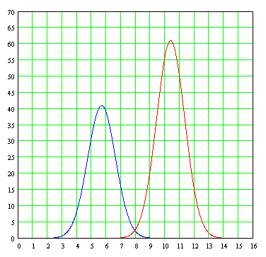
then if we can "force" the data to fall within a formula modeled on a continuous independent variable whose stroke is "fit" to the heights of the bars of the histograms, obtaining in this last example a setting like this (this adjustment is carried out simply by adding the expressions for two Gaussian curves with means other than by changing individual variances and amplitudes of each curve to the score):

this setting is a setting meaningless, since a chart like this, known as graphical bimodal, which has two "caps" peaks, is telling us that instead of having a population of data the same source we have is two populations of different origins data, data that came tucked into a single "package" at the hands of the analyst. This is when the analyst is almost forced to go to the "field" to see how and where data were collected. It is possible that the data represent the lengths of certain beams which were produced by two different machines. It is also possible These data have originated in an experiment in which he was testing the effect of a new type of fertilizer on yield of some crops and the fertilizer was being supplied to experimental plots for two different people in two different places, in which case there something that is causing a significant difference in the performance of the fertilizer and the effect it may have the fertilizer itself, either that both persons have been supplying different quantities of the same fertilizer, or the characteristics of different areas have caused Gaussian distribution altered the performance of each type of fertilizer.
For the continuous curve "double hump" shown above, this curve was drawn by the following formula score obtained by adding two Gaussian curves and setting the "top" of each curve to match the approximate-manipulating the arithmetic mean μ at each end-caps with each of the two top bars, modifying also the variance σ in each term for "open" or "close" the width of each fitted curve will:

Then we separated individual plots (not added) to each of the Gaussian curves shown in the formula, showing a probable range of data from two distinct populations of which came from the scrambled data.

In this example, it was easy to just view the histogram, the bar graph data-the presence of two Gaussian curves instead of one, thanks to the arithmetic mean of each curve (5.7 and 10.4) are separated by a margin of almost two to one. But we will not always so lucky, and there will be cases in which the arithmetic will be so close to each other that will be somewhat difficult for the analyst to decide if it considers all data as one or try to find two different curves, as would occur with a graph whose curve joining the heights of the bars would look like this:

is in cases like these in which the analyst must draw on all her wit and all his experience to decide if he tries to find two discernible groups of data in the data set at hand, or if it is not worth for the presence of two distinct populations riots in one, opting to perform modeling based on a single Gaussian formula.
Discovering the influence of unknown factors that may affect the performance of something as a fertilizer is just one of the primary objectives the design of experiments . In the design of experiments are not interested in carrying out a modeling of the data to a formula, that comes after it has been established unequivocally how many and what are the factors that can affect performance or response to something. Once passed this stage, we can collect data to carry out the adjustment of data to a formula. In the case of a bimodal distribution, instead of trying to set a formula to describe all data with a single distribution as we have seen, is much better to try to separate the data from the two different populations that are causing the "double hump camel ", a fact that can analyze two data sets separately with the assurance that for each data set we obtain a Gaussian distribution with a single hump. It can be seen from this that the formulas data modeling is a continuous cycle experimentation, analysis and interpretation of results, followed by a new cycle of experimentation and analysis and interpretation of new results to be improving a process or could go better describing the data being collected in a laboratory or field. The data modeling formula goes hand in hand with the procedures for the collection of the same.
PROBLEM : experimentally in the laboratory is the boiling point for some organic compounds known as alkanes (chemical formula C n H 2n +2 \u200b\u200b ) has the following values \u200b\u200bin degrees Celsius:
Methane (1 carbon atom): -161.7
ethane (2 carbons): -88.6
propane (3 carbon atoms): -42.1
butane (4 carbons): -0.5
pentane (5 carbon atoms): 36.1
hexane (6 carbon atoms): 68.7
heptane (7 carbons): 98.4
octane (8 carbon atoms): 125.7
Nonane (9 carbon atoms): 150.8
Dean (10 carbon atoms): 174.0
Make a graph of the data. Does it show any tendency the boiling point of these organic compounds according to the number of carbon atoms that have each compound?
The graph of discrete data is as follows:

The graph we can see that the data seem to accommodate a super smooth continuous curve, following the cause-effect, which we suggests that behind this data is a natural law waiting to be discovered by us. Since the data do not follow a straight line, the relationship between them is not a linear relationship, is a non-linear relationship , and do not expect that the mathematical formula that is behind this curve is that of a line straight. In the absence of a theoretical model that allows us to have the exact formula, the graph arising from this data set is an excellent example of the places where we can try to adjust the data to an empirical formula, the better the data fit , the better we will suggest the nature of natural laws operating behind this phenomenon.
PROBLEM: Given the following distribution of the diameters of the heads of rivets (expressed in inches) made by some company and the frequency f with which they occur:

representative a total of 250 measurements, adjusting a Gaussian curve to these data. Also, make the outline of a bar graph of the data superimposing Gaussian curve on the same graph.
For Gaussian curve, the first step is to obtain the arithmetic mean of the data:

By the way which are presented the data, we have to make a slight modification in our calculations to obtain the arithmetic mean of the same, using as the representative value of each interval the average value between the minimum and maximum of each interval. Thus, the representative value in the range between .7247 and .7249 is .7248, the representative value in the range between .7250 and .7252 is .7251, and so on. Each of these values \u200b\u200brepresenting each interval weight we must give "fair" that belongs in the calculation of the mean multiplied by the frequency with which it occurs. Thus, the value .7248 will be multiplied by 2 since this is the frequency con la cual ocurre, y el valor .7251 será multiplicado por 6 puesto que esa es la frecuencia con la cual ocurre, y así sucesivamente. De este modo, la media aritmética de la población de 250 datos será:
Tras esto obtenemos la desviación estándard σ calculando primero la varianza σ 2, also using in our calculations here the representative values \u200b\u200bof each interval and the frequency with which each such case values:
With this we all we need to produce the Gaussian curve fitted to the data. The height of the curve is selected to coincide with the bar (representing Data Range), which also has the highest, which is still the diameter range between .7262 and .7264 inches with a "height" of 68 units. Thus, the graph, using a "high" for the Gaussian curve of 68 units is as follows:

The Gaussian curve fit to the data does not seem as "ideal" as we wanted. This is about something more fundamental than the fact that the arithmetic mean X of data (72 642 inches) is not identical to the representative point of the range of values \u200b\u200b(7263) in which it occurs as often of the 68 observations ( and emphasized here as being of greater importance than in real life is very rare time in which the maximum of the calculated curve coincides with the arithmetic value is more likely to be the arithmetic average ) , let alone the fact that the bar chart has been drawn without each bar extends to touch with its neighboring bars. If you look around the distribution of the data, we see that the distribution data are more loaded bar to the right than left. Ideal Gaussian curve we have been driving is a perfectly symmetrical curve, with the same amount of data or observations distributed to the right of the vertical axis of symmetry to the left. This asymmetry is known as bias ( skew) or lean precisely because the original data is loaded more than one side than the other, that is precisely what makes the "top" of the distribution of rods in graph does not coincide with the arithmetic mean of the data. And although there is a theorem in statistics called the Central Limit Theorem (Central Limit Theorem ) tells us that the sum of a large number of independent random variables will be normally distributed (Gaussian) with increasing amount data or observations, taking more and more readings will not necessarily make the data are adjusted to become more symmetrical curve, this will not happen if there are substantive reasons why more data is loaded to one side than the other. This is a situation that the ideal Gaussian curve is not prepared to handle, and if we want to accurately adjust a curve to data in which we would expect an ideal Gaussian behavior then we need to modify the Gaussian curve becoming more complex formula, using a the multiply trick as the amplitude of the curve by some factor that makes their decline is not as "soft" either right or left. Unfortunately, the use of such tricks are often no theoretical justifications to explain the amendment to the modeled curve, are simply a resource for fine adjustment. This is when the experimenter or data analyst has to decide if the goal is really trying to justify the resort to such tricks, but have their way, do not help improve our understanding of what is happening behind a accumulation of data. There

representative a total of 250 measurements, adjusting a Gaussian curve to these data. Also, make the outline of a bar graph of the data superimposing Gaussian curve on the same graph.
For Gaussian curve, the first step is to obtain the arithmetic mean of the data:

By the way which are presented the data, we have to make a slight modification in our calculations to obtain the arithmetic mean of the same, using as the representative value of each interval the average value between the minimum and maximum of each interval. Thus, the representative value in the range between .7247 and .7249 is .7248, the representative value in the range between .7250 and .7252 is .7251, and so on. Each of these values \u200b\u200brepresenting each interval weight we must give "fair" that belongs in the calculation of the mean multiplied by the frequency with which it occurs. Thus, the value .7248 will be multiplied by 2 since this is the frequency con la cual ocurre, y el valor .7251 será multiplicado por 6 puesto que esa es la frecuencia con la cual ocurre, y así sucesivamente. De este modo, la media aritmética de la población de 250 datos será:
X = [2∙(.7248) + 6∙(.7251) + 8∙(.7254) + ... + 4∙(.7278) + 1∙(.7281)]/250
X = 181.604/250
X = .72642 pulgadas
X = 181.604/250
X = .72642 pulgadas
Tras esto obtenemos la desviación estándard σ calculando primero la varianza σ 2, also using in our calculations here the representative values \u200b\u200bof each interval and the frequency with which each such case values:
Σd ∙ ² = 2 (-. 7248 72 646) ² + 6 (7251 -. 72 642) ² + ... + 1 ∙ (.7281 -. 72 642) ²
Σd ² = 0.000082926
σ = Σd ² ² / N = 0.00008292/250 = 0.000000331704
σ = .00057594 inches
Σd ² = 0.000082926
σ = Σd ² ² / N = 0.00008292/250 = 0.000000331704
σ = .00057594 inches
With this we all we need to produce the Gaussian curve fitted to the data. The height of the curve is selected to coincide with the bar (representing Data Range), which also has the highest, which is still the diameter range between .7262 and .7264 inches with a "height" of 68 units. Thus, the graph, using a "high" for the Gaussian curve of 68 units is as follows:

The Gaussian curve fit to the data does not seem as "ideal" as we wanted. This is about something more fundamental than the fact that the arithmetic mean X of data (72 642 inches) is not identical to the representative point of the range of values \u200b\u200b(7263) in which it occurs as often of the 68 observations ( and emphasized here as being of greater importance than in real life is very rare time in which the maximum of the calculated curve coincides with the arithmetic value is more likely to be the arithmetic average ) , let alone the fact that the bar chart has been drawn without each bar extends to touch with its neighboring bars. If you look around the distribution of the data, we see that the distribution data are more loaded bar to the right than left. Ideal Gaussian curve we have been driving is a perfectly symmetrical curve, with the same amount of data or observations distributed to the right of the vertical axis of symmetry to the left. This asymmetry is known as bias ( skew) or lean precisely because the original data is loaded more than one side than the other, that is precisely what makes the "top" of the distribution of rods in graph does not coincide with the arithmetic mean of the data. And although there is a theorem in statistics called the Central Limit Theorem (Central Limit Theorem ) tells us that the sum of a large number of independent random variables will be normally distributed (Gaussian) with increasing amount data or observations, taking more and more readings will not necessarily make the data are adjusted to become more symmetrical curve, this will not happen if there are substantive reasons why more data is loaded to one side than the other. This is a situation that the ideal Gaussian curve is not prepared to handle, and if we want to accurately adjust a curve to data in which we would expect an ideal Gaussian behavior then we need to modify the Gaussian curve becoming more complex formula, using a the multiply trick as the amplitude of the curve by some factor that makes their decline is not as "soft" either right or left. Unfortunately, the use of such tricks are often no theoretical justifications to explain the amendment to the modeled curve, are simply a resource for fine adjustment. This is when the experimenter or data analyst has to decide if the goal is really trying to justify the resort to such tricks, but have their way, do not help improve our understanding of what is happening behind a accumulation of data. There
experiments in which although it is tempting to immediately get a formula of "best fit" to a series of data, such a formula will do little to reach a conclusion or really important discovery that can be removed with a little cunning in the study of the accumulated data. An example is the following problem (problem 31) taken from chapter 27 (The Electrical Field) of the book "Physics for Engineering and Science Students" by David Halliday and Robert Resnick
PROBLEM: One of his first experiments (1911) Millikan found that, among other charges, appeared at different times as follows, measured at a particular drop:
6,563 • 10 -19 coulombsWhat value of elementary charge can be deduced from these data? Accommodating
8,204 • 10 -19 coulombs
11.50 • 10 -19 Coulombs
13.13 • 10 -19 coulombs
16.48 • 10 -19 coulombs
18.08 • 10 -19 coulombs
19.71 • 10 -19 coulombs
22.89 • 10 -19 coulombs
26.13 • 10 -19 coulombs
data in increasing order of magnitude, we can make a graph of them who happens to be the next (this chart and other productions in this work can be seen more clearly or even in some cases expanded with the simple expedient of enlarge):

is important to note that this chart is not an independent variable (whose value would be placed on the horizontal axis) and a dependent variable (whose value would be placed on the vertical axis) as the horizontal axis simply been assigned a different ordinal number to each of the experimental values \u200b\u200blisted, so the first item (1) has a value of 6,563 • 10 -19 , the second data (2) has a value of 8,204 • 10 -19 , and so on.
We can, if we want to obtain a straight line of best fit for these hand-drawn data. But this entirely misses the perspective of the experiment. A chart much more useful than the dot plot shown above is the following graph of the data known as graphical ladder or step graphical :

carefully inspecting the graph of this data, We realize that there are "steps" which seems to be the same height of a datum to the next. The difference between observations 1 and 2, for example, seems to be the same as the difference between observations 6 and 7. And those "gaps" where it is not, seems to be height twice the height other steps. If the height of a step to the next did not have this similarity with any of the remaining observations, we may conclude that the differences are completely random. But this is not what is happening and the steps seem to have heights equal to or double equal. These data are revealing something important, that electric charge is quantized , the electric charge reported here does not vary much from 0.7, 1.4 or 2.5, but integral multiples of one or two goals. The data we are confirming the existence of the electron , the smallest electric charge is no longer possible subdivided by physical or chemical means at our disposal. Among the data on which the "jump" from one step to another is double from that in other steps, we can conclude that data are "missing" and that an additional amount of experiments, it should be possible to find experimental values \u200b\u200bbetween those jumps "doubles" that posts in the graph, we must produce a staircase with steps of similar height could be called "basic." By way of example, the reported value of 11.50 • 10 -19 coulombs and 8,204 • 10 -19 coulombs must have an intermediate value of about 9,582 • 10 -19 coulombs with an additional recabación laboratory data should be possible to detect sooner or later.
We can estimate the magnitude of the electric charge as we now know as the electron by first obtaining the differences between the data representing a unit jump by averaging them, and after that the differences between the data representing a jump "double" also getting the same average and dividing the result of the latter two, summing and averaging the two sets of values \u200b\u200band for a final result:
Set 1 (Jump Unit):
8204 • 10 -19 - 6,563 • 10 -19 = 1,641 • 10Joint 2 (Double Jump):
-19 13.13 -19 • 10 - 11.50 • 10 -19 = 1.63 • 10 -19
18.08 • 10 -19 - 16.48 • 10 -19 = 1.6 • 10
-19 19.71 -19 • 10 - 18.08 • 10 -19 = 1.63 • 10 -19
11.50 • 10 -19 - 8204 • 10 -19 = 3,296 • 10 -19The average first set of data is:
16.48 • 10 -19 - 13.13 • 10 -19 = 3.35 • 10 -19
22.89 • 10 -19 - 19.71 • 10 -19 = 3.18 • 10 -19
26.13 • 10 -19 - 22.89 • 10 -19 = 3.24 • 10 -19
(1,641 • 10 -19 + 1.63 • 10 -19 + 1.6 • 10 -19 + 1.63 • 10 -19 ) / 4 = 1625 • 10 -19 coulombs
And the average of the second data set is:
(3376 • 10 -19 + 3.35 • 10 -19 + 3.18 • 10 -19 + 3.24 • 10 -19 ) / 4 = 3.2655 • 10 -19
that it be divided into two:
3.2655 • 10 -19 / 2 = 1633 • 10 -19 coulombs
Since there are so many data ( 4 data) in the first set and in the second set, we can give the same "simple weight" to each of the averages obtained by adding the average first to second average and dividing the result by two (of not being so, both teams have had a different number of observations, we have to give a "significant factor" arithmetic each set to give each contribution according to their relative importance):
(1,625 • 10 -19 + 1633 • 10 -19) / 2 = 1.63 • 10 -19 coulombs
As a postscript to this problem, which is added later experiments conducted with greater precision and minimizing sources of error with a seeking of a large number of data (which helps to gradually reduce the random error due to causes beyond the control of the experimenter) leads to a more accurate value of 1.60 • 10 -19 coulombs for the electron charge, which is the accepted value today.
This problem points out that, before attempting to adjust a set of experimental data to a formula, is important to carefully consider the graph of the data to see if we are missing something very important that the data are telling us. It may not even be of importance or of no use to try to obtain a formula fitted to the data under such conditions.
Saturday, March 29, 2008
Mr Men T-shirts Singapore
2: The linear fit formulas
easier adjustment formula data that we can carry out is one in which the data show a linear trend in which the data appear to follow a trend in a straight line when placed on a graph. The first step, before anything, is to translate data into a graph at our disposal to determine if indeed there is any trend (either linear or nonlinear) for grouped data following a certain trend, behind which there is possibly a natural relationship that eventually can be expressed with a simple formula. If the graph of the data from several pairs of measurements of two variable quantities, of which perhaps can be varied at will, this is a as follows:

we can see that there seems to be no correlation between the graphed data. However, if the graph turns out to be one like this:

then it manifests as a tendency. These data, allegedly obtained by experiment, usually to be affected with a random error (occurring at random) denoted by the Greek letter ε (equivalent to the Latin letter "e"). If it were not for this error, possibly all the data fall in a straight line or a smooth, continuous curve of the phenomenon itself is being described by the data. In the last graph, it is tempting to draw "by hand" on the same straight line as close as possible to our data, a straight line like the following:

The problem with a plot "by hand" of the straight line is that different people get different lines according to their own subjective criteria, and possibly no one will have the same line, having no way of knowing which of them is the best. That is why, in order to unify criteria and get the same answer in all cases, we need to use a mathematical approach . This approach gives us the method of least squares , developed by the "prince of mathematics" Carl Friedrich Gauss.
The idea behind the method of least squares is as follows: if on a dataset in a graph that seem to cluster along a trend marked by a straight line is drawn a straight line, then all the different lines that can be drawn we can try to find one which produces "best fit" (in English this is called best fit) of according to some mathematical criterion. This line may be that such that the "average distance" from all points on the graph to the ideal line is the smallest average distance possible. Although the distances of each point to the ideal line can be defined so as to be perpendicular to the line, as shown in the picture below right:

mathematical manipulation of the problem can be greatly simplified if instead of using such distances perpendicular to the ideal use vertical distances as the vertical axis of the graph as shown in the picture above left.
While we could try to use absolute values \u200b\u200b d │ i │ distances of each of the points i to the ideal line (the absolute values \u200b\u200beliminate the presence of negative values \u200b\u200baveraged over the Positive values \u200b\u200bwould end "canceling" We intend to obtain a useful average), the main problem is that the absolute value any variable can not be differentiated mathematically in a conventional manner, not easily lend itself to a mathematical derivation using the usual resources of differential calculus, which is a disadvantage when they go to use the tools of the calculation to obtain the maximum and minimum. That is why we use the sum of the squares distances rather than the absolute values \u200b\u200bof the same, as this allows us to treat these securities, known as residual , as a quantity continuously differentiable. However, this technique has the disadvantage that when used square of the distance those isolated points are very far from the ideal line will have an effect on the setting, something that we should not lose sight of when they appear isolated in the graph data that seem too far from the ideal line and which may be indicative of a mistake in measurement or bad data recorded.
For data that seem to show a linear trend, according to the method of least squares is assumed from the outset the existence of a line "ideal" that provides the best fit (best fit ) known as "least-squares fit (least squares fit ). The equation of this "ideal line" is:
where A and B are the parameters (constant number) to be determined under the criterion of least squares.
Given a number N of pairs of experimental points (X 1 , And 1), (2 X, Y 2), (X 3 , And 3), etc., then for each experimental point corresponding to each value of the independent variable X = X 1 , X 2, X 3 ,..., X N be a calculated value and i = and 1 , and 2, and 3 ... using the straight "ideal", which is:
The difference between real value of Y = Y 1 , Y 2, and 3 ,..., Y N and each value calculated for the corresponding X i using the ideal line gives us the "distance" vertical D i that alienates both values:
Each of these distances D i is known in mathematical statistics as the residual .
straight To find the "ideal", we will use the established procedures of differential calculus for determining the maximum and minimum. A first attempt to lead us to try and find the line that minimizes the sum of the distances
However, this scheme will not serve us much, because the calculations to determine the value of each distance D i some points "real" above the line will and others will be below it, which some of the distances are positive and some negative (possibly distributed in equal parts) thus canceling much of their contributions the construction of the function you want to minimize. This leads us immediately to try to use absolute values \u200b\u200b distances:
3 ² + ... + D N ²
2) ² + (A + BX 3
The solution of these equations gives us the equations required:
AN + B Σ
X -
Σ Y = 0

Σ A X + B
And

A
Σ
X + B
PROBLEM:
Given the following, obtain the line of least squares:

To use the equations required to obtain the line of least squares, it is desirable to accommodate the summation in a table like the one shown below:
From this table of intermediate results we obtain:
(
X ²
)
Σ
X ² -
see that the fit is reasonably good. And, most important, other researchers will get exactly the same result under the criterion of square Mimin such problems. Significantly, the mechanization of the evaluation of these data by columns such as arrangements that were used up getting
Σ
and
X ² Σ XY 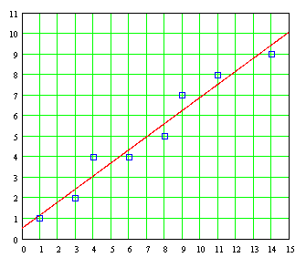 can be done in a "worksheet" as EXCEL.
For a large set of data pairs, other times these calculations used to be tedious and subject to mistakes. Fortunately, with the advent of programmable pocket calculators and computer programs that can now be performed on a desktop computer arithmetic for which only two decades ago required expensive computers and sophisticated software in a scientific programming language such as FORTRAN These calculations can be machined to such an extent that instead of having to use excessive amounts of time in performing the calculations the emphasis today is on and l analysis and interpretation of results
. If, on the basis of experimental data or data obtained from a sample taken from a population we want to estimate the value of a variable Y corresponding to a value of another variable X from the least-squares curve best fits the data, it is customary to call the resulting curve the regression curve of Y in X since And is estimated X . If the curve is a straight line, then call that line the regression line of Y on X . An analysis carried out by the method of least squares is also called regression analysis, and computer programs that can perform calculations are called least-squares regression programs
. If, however, instead of estimating the value of
And
from X value we wish to estimate the value of X from And then we would use a curve regression of X on Y , which involves simply exchanging the variables in the diagram (and in the normal equations) so that X is the dependent variable and And the independent variable, which in turn means replacing the vertical distances D used in the derivation of the least squares line for horizontal distances :
An interesting detail is that, generally, for a given set of data the regression line in X Y and the regression line in X Y two different lines that do not match exactly in a diagram, but in any case are so close to each other that could be confused.
PROBLEM:
a) Get the regression line of Y on X, given Y as the dependent variable and X as independent variable. b)
Get the regression line of X on Y, given X and Y as the dependent variable as independent variable.
a) Considering Y as the dependent variable and X as the independent variable, the equation of the least squares line is Y = A + BX, and the normal equations are: BΣX ΣY = AN +
ΣXY = AΣX + BΣX ² 8A + 56B = 40
56A + 524B = 364
Simultaneous two equations, we get A = 6 / 11 and B = 7 / 11. Then the least squares line is:
Y = 6 / 11 + (7 / 11) X
Y = 0.545 + 0.636 X
b) Considering X as the dependent variable and Y as independent variable, the least squares equation is now X = P + QY, and normal equations are:
sx = PN + QΣY
8P +
X = -0.5 + 1.5Y
For comparative purposes, we can solve this formula to make And depending on X, obtaining:
Y = 0.333 + 0.667 X
We note that the regression lines obtained in (a) and (b)
different. Below is a chart showing the two lines:
An important measure of how well is the "adjustment" of various experimental data to a straight line obtained from the minimum by the method of least squares is the correlation coefficient
. When all the data is located exactly on a straight line, then
correlation coefficient is unity, and as data on a graph will show increasingly dispersed in relation to the line then the correlation coefficient gradually decreases as shown by the following examples:
As a courtesy of Professor Victor Miguel Ponce, professor and researcher at San Diego State University are available to the public on his personal website on the Internet several programs to machine calculations required to "adjust" data set with a linear trend line of "least squares". The page that provides all programs is:
To use the above program, we introduce first the size of the array (array ), or the amount of data pairs, after which we introduce the values \u200b\u200b
paired data in an orderly manner starting first with the values \u200b\u200bseparated by commas, followed by the values \u200b\u200bof x, also separated by commas. Done, press "Calculate" at the bottom of the page, which we obtain the values \u200b\u200bα
, the correlation coefficient
r
The standard error
estimation and dispersions (standard deviations) σ
x and σ and data x i and data and i . As an example of using this program, we obtain the least squares line for the following pairs of data: x (1) = 1 and (1) = 5 x (2) = 2, and ( 2) = 7 x (3) = 4, and (3) = 11 x (4) = 5, and (4) = 13 x (5) = 9, and (5) = 21 De Under this program, least squares line is: Y = 3 + 2X And the correlation coefficient r is
= 1.0, while the standard error of the estimate is zero, which as we shall see later tells us that
all pairs of data are part of the line of least squares
. If we plot the least squares line and plotted on it the data pairs (x
i
,
and
which confirms that the mathematical criterion that we used to get the line of least squares, we have defined the correlation index r are correct, we have defined the standard error of the estimate is correct . far we have considered a "least-squares fit" associated with a line that might be called "ideal" from a mathematical point of view, where we have an independent variable (cause) that produces an effect on some dependent variable (effect) . But it may be the case we have a situation in which some variable values \u200b\u200btake will be dependent on not one but two or more factors. In this case, if the individual unit because each of the factors, keeping the other constant, is a linear dependence, we can extend the method of least squares to cover this situation as we did when there was only one variable independent. This is known as a multiple linear regression . For two variables X and X 1 2, this dependence is represented as Y = f (X
1, X 2
In this graph, the height of each point represents the value of Y for each each pair of values \u200b\u200bX and X
1 2. Representing the points without explicitly show the "highest" points to the horizontal plane Y = 0, making three-dimensional graph like this:
The least squares method used to adjust a set of data to a least squares line can also be extended to obtain a formula of least squares, in which case for two variables the regression equation will the following:
1 X 1 + A 2 X 2
 and often erroneously, this equation is taken as representing a line. However, there is a line, is a surface
. If we perform a least squares fit on the linear formula with two factors X and X 1
2, we obtain what is known as a regression
If we get the equations for this least squares plane , we proceed in exactly the same way as we did to get the formulas which evaluate the parameters to obtain the least squares line, that is, we define the vertical distances of each of the ordered pairs of points into this plane of least squares:

By extension, the problems involving more than two variables and
1 X 2
, suppose we start with a relationship between the three variables that can be described by the following formula:
 Y = α
Y = α
+ ß 1 X
1 + ß 2 X 2
which is a linear formula in the variables
2. values \u200b\u200band in this line correspond to X 1 = X 1 1 , X 1 2 , X 1 3. .. , X 1 N and 2 X = X 2 1, X 2 2, X 2 3 .. . , X 2 N (we use here the subscript to distinguish each of the two variables X and 1 X 2, and superscript to eventually perform summation over the values \u200b\u200bto each of these variables) are α + ß 1 X 1 1 + ß 2 X 2 1 , α + ß 1 X 1 2 + ß 2 2 X 2 , α + ß 1 X 1 3 + ß 2 X 2 3 ... , Α + ß 1 X 1 N + ß 2 X 2 N , while current values \u200b\u200bare And 1 , Y 2, 3 And ... , And N respectively. Then, as we did on the regression equation based on a single variable, we define the "gap" produced by each trio of experimental data to values \u200b\u200b And i so that the sum of the squares of these distances is: S = (α + ß 1 1 X 1 + ß 2 X 2
Proceeding as we did when we had two parameters instead of three, this gives us the following set of equations: N α + ß 1 Σ X
1
X
2
. There is a reason why these equations are called normal equations. If we represent the data set for the variable X 1 as a vector X 1 and data set for the variable X 2 as another vector X
2
, considering that these vectors are independent of each other (using a term from linear algebra, linearly independent, which means they are not a simple multiple of each other physically pointing in the same direction) then we can put these vectors in a plane. On the other hand, we consider the sum of squared differences D i used in the derivation of normal equations as well as the magnitude of a vector D i , recalling that the square length of a vector is equal to the sum of the squares of its elements ( an extended Pythagorean theorem dimensions). This makes the principle of "best fit" is equivalent to find one difference vector D i corresponding to the shortest possible distance to the plane formed by vectors X 1 X and 2 . And the shortest distance possible is a vector perpendicular or normal vector : the plane defined by vectors X and 1 X 2 (or rather, the plane formed by the linear combination of vectors ß 1 X
X2). Although we can repeat here the formulas that correspond to the case of two variables X and 1 X 2 , having understood what a "flat of square Mimin "we can use one of many commercially available computer programs or online. The personal page of Professor Victor Miguel Ponce quoted above gives us the means to carry out a" least-squares fit "when it comes to case of two variables X and 1 X 2 , accessible at the following address: http://ponce.sdsu.edu/onlineregression13.php
PROBLEM: Getting the formula plane that best fits the representation of the following data set: These data, represented in three dimensions, are the following aspect:
For this data set, the formula that corresponds to the surface regression is:
1
2
Y = -2
X1 and X2 are varied from -10 to +10 and dimensional graph is rotated around the axis turning And, why this kind of graphs are known under the name "spin plot" (requires enlarge to see the animated action):
Y = ß 0 + ß 1 X
X
2
1 X 1
+ ß 2 X
2
and 1 ß 2 this interaction could be of such magnitude could even nullify the importance of the variable terms ß 1 X 1 and ß 2 X 2 . This issue alone is large enough to require to be dealt with separately in another section of this work.
The idea behind the method of least squares is as follows: if on a dataset in a graph that seem to cluster along a trend marked by a straight line is drawn a straight line, then all the different lines that can be drawn we can try to find one which produces "best fit" (in English this is called best fit) of according to some mathematical criterion. This line may be that such that the "average distance" from all points on the graph to the ideal line is the smallest average distance possible. Although the distances of each point to the ideal line can be defined so as to be perpendicular to the line, as shown in the picture below right:

mathematical manipulation of the problem can be greatly simplified if instead of using such distances perpendicular to the ideal use vertical distances as the vertical axis of the graph as shown in the picture above left.
While we could try to use absolute values \u200b\u200b d │ i │ distances of each of the points i to the ideal line (the absolute values \u200b\u200beliminate the presence of negative values \u200b\u200baveraged over the Positive values \u200b\u200bwould end "canceling" We intend to obtain a useful average), the main problem is that the absolute value any variable can not be differentiated mathematically in a conventional manner, not easily lend itself to a mathematical derivation using the usual resources of differential calculus, which is a disadvantage when they go to use the tools of the calculation to obtain the maximum and minimum. That is why we use the sum of the squares distances rather than the absolute values \u200b\u200bof the same, as this allows us to treat these securities, known as residual , as a quantity continuously differentiable. However, this technique has the disadvantage that when used square of the distance those isolated points are very far from the ideal line will have an effect on the setting, something that we should not lose sight of when they appear isolated in the graph data that seem too far from the ideal line and which may be indicative of a mistake in measurement or bad data recorded.
For data that seem to show a linear trend, according to the method of least squares is assumed from the outset the existence of a line "ideal" that provides the best fit (best fit ) known as "least-squares fit (least squares fit ). The equation of this "ideal line" is:
Y = A + BX
where A and B are the parameters (constant number) to be determined under the criterion of least squares.
Given a number N of pairs of experimental points (X 1 , And 1), (2 X, Y 2), (X 3 , And 3), etc., then for each experimental point corresponding to each value of the independent variable X = X 1 , X 2, X 3 ,..., X N be a calculated value and i = and 1 , and 2, and 3 ... using the straight "ideal", which is:
and 1 = A + BX 1
and 2 = A + BX 2
and 3 = A + BX 3
.
.
.
and N = A + BX N
and 2 = A + BX 2
and 3 = A + BX 3
.
.
.
and N = A + BX N
The difference between real value of Y = Y 1 , Y 2, and 3 ,..., Y N and each value calculated for the corresponding X i using the ideal line gives us the "distance" vertical D i that alienates both values:
D 1 = A + BX 1 - Y 1
2 D = A + BX 2 - And 2
D 3 = A + BX 3 - Y 3
.
.
.
D N = A + BX N - Y N
2 D = A + BX 2 - And 2
D 3 = A + BX 3 - Y 3
.
.
.
D N = A + BX N - Y N
Each of these distances D i is known in mathematical statistics as the residual .
straight To find the "ideal", we will use the established procedures of differential calculus for determining the maximum and minimum. A first attempt to lead us to try and find the line that minimizes the sum of the distances
S = D 1 + D + D 2 3 + ... D + N
However, this scheme will not serve us much, because the calculations to determine the value of each distance D i some points "real" above the line will and others will be below it, which some of the distances are positive and some negative (possibly distributed in equal parts) thus canceling much of their contributions the construction of the function you want to minimize. This leads us immediately to try to use absolute values \u200b\u200b distances:
S = another scheme in which we also add the distances D i but without the problem of mutual cancellation of terms having positive and negative terms. The strategy is to use squares of the distances: S = D 1 D ² + 2 ² + D
3 ² + ... + D N ²
With this definition, the general term we want to minimize is given by: S = (A + BX 1 And 1 ) ² + (A + BX 2 And
2) ² + (A + BX 3
And 3) ² + ... + (A + BX N-Y N ) ² The unknowns of the line we are looking for are ideal parameters and A B . With respect to these two questions is how we must carry out the minimization of S . If it were a single parameter, a sufficient ordinary differentiation. But since there are two parameters, we must carry out two separate distinctions derived using partial in which we differentiate with respect to a parameter keeping the other constant. from the calculation, S be a minimum when the partial derivatives with respect to A and B are zero. These partial derivatives are:
The solution of these equations gives us the equations required:
AN + B Σ
X -
Σ Y = 0

Σ A X + B
Σ X ² - Σ XY = 0
where we are using the following simplified symbolic notation:
where we are using the following simplified symbolic notation:
The two equations we can rearrange as follows: AN + B Σ X =
Σ And

A
Σ
X + B
Σ X ² = Σ XY
taking with it two equations linear which can be solved as simultaneous equations either directly or through the method of Cramer (determinants), thus obtaining the following formulas:
taking with it two equations linear which can be solved as simultaneous equations either directly or through the method of Cramer (determinants), thus obtaining the following formulas:
Thus, the substitution of data in the two formulas give us the values \u200b\u200bof the parameters and A B we are looking for and the "ideal line, the line provides the best fit of all that we can draw on the criteria we defined. Since we are minimizing a function that minimizes the sum of the squares of the distances (residuals), this method as mentioned above is known universally as the method of least square.
PROBLEM:
Given the following, obtain the line of least squares:

To use the equations required to obtain the line of least squares, it is desirable to accommodate the summation in a table like the one shown below:
From this table of intermediate results we obtain:
(
Σ  And
And
) (
Σ  And
And ) (
X ²
)
- (Σ 
X) ( Σ 
XY) = (40) (524) - (56) (364) = 6 N Σ XY - (X Σ) (Σ And ) = (8) (364) - (56) (40) = 7 N
Σ
X ² - ( Σ X ) ² = (8) (524) - (56 ) ² = 11 And using the above formulas obtained:
A = [
( AND Σ) (Σ X ² ) - ( Σ
X) (XY Σ
X ² - ( Σ X ) ² = (8) (524) - (56 ) ² = 11 And using the above formulas obtained:
A = [
( AND Σ) (Σ X ² ) - ( Σ
Σ
) ] / [N Σ X ² - (Σ X ) ²] = 6 / 11 A = .545 B = [N Σ XY - ( Σ X ) ( Σ
And
) ] / [N
Σ
And
) ] / [N
Σ
X ² -
( Σ X ) ²] = 7 / 11 B = .636 The least squares line is then: Y = A + BX Y = 0.545 + 0.636 X The graph of this straight line superimposed on the individual point pairs is:
We see that the fit is reasonably good. And, most important, other researchers will get exactly the same result under the criterion of square Mimin such problems. Significantly, the mechanization of the evaluation of these data by columns such as arrangements that were used up getting
Σ
X, Y
Σ , Σ
Σ , Σ
and
X ² Σ XY
 can be done in a "worksheet" as EXCEL.
 For a large set of data pairs, other times these calculations used to be tedious and subject to mistakes. Fortunately, with the advent of programmable pocket calculators and computer programs that can now be performed on a desktop computer arithmetic for which only two decades ago required expensive computers and sophisticated software in a scientific programming language such as FORTRAN These calculations can be machined to such an extent that instead of having to use excessive amounts of time in performing the calculations the emphasis today is on and
. If, on the basis of experimental data or data obtained from a sample taken from a population we want to estimate the value of a variable Y corresponding to a value of another variable X from the least-squares curve best fits the data, it is customary to call the resulting curve the regression curve of Y in X since And is estimated X . If the curve is a straight line, then call that line the regression line of Y on X . An analysis carried out by the method of least squares is also called regression analysis, and computer programs that can perform calculations are called least-squares regression programs
. If, however, instead of estimating the value of
And
from X value we wish to estimate the value of X from And then we would use a curve regression of X on Y , which involves simply exchanging the variables in the diagram (and in the normal equations) so that X is the dependent variable and And the independent variable, which in turn means replacing the vertical distances D used in the derivation of the least squares line for horizontal distances :
An interesting detail is that, generally, for a given set of data the regression line in X Y and the regression line in X Y two different lines that do not match exactly in a diagram, but in any case are so close to each other that could be confused.
PROBLEM:
Given the following data set: 

a) Get the regression line of Y on X, given Y as the dependent variable and X as independent variable. b)
Get the regression line of X on Y, given X and Y as the dependent variable as independent variable.
a) Considering Y as the dependent variable and X as the independent variable, the equation of the least squares line is Y = A + BX, and the normal equations are: BΣX ΣY = AN +
ΣXY = AΣX + BΣX ² 8A + 56B = 40
 Carrying out the summation, the normal equations become:
 56A + 524B = 364
Simultaneous two equations, we get A = 6 / 11 and B = 7 / 11. Then the least squares line is:
Y = 6 / 11 + (7 / 11) X
Y = 0.545 + 0.636 X
b) Considering X as the dependent variable and Y as independent variable, the least squares equation is now X = P + QY, and normal equations are:
sx = PN + QΣY
ΣXY = PΣY + QΣY ²
Carrying out the summation, the normal equations become:
Carrying out the summation, the normal equations become:
8P +
40Q = 56 = 364 40P + 256Q Simultaneous
both equations, we obtain P =- 1 / 2 and Q = 3 / 2. Then the least squares line is:
X = -1 / 2 + (3 / 2) Y both equations, we obtain P =- 1 / 2 and Q = 3 / 2. Then the least squares line is:
X = -0.5 + 1.5Y
For comparative purposes, we can solve this formula to make And depending on X, obtaining:
Y = 0.333 + 0.667 X
We note that the regression lines obtained in (a) and (b)
different. Below is a chart showing the two lines:
An important measure of how well is the "adjustment" of various experimental data to a straight line obtained from the minimum by the method of least squares is the correlation coefficient
correlation coefficient is unity, and as data on a graph will show increasingly dispersed in relation to the line then the correlation coefficient gradually decreases as shown by the following examples:
As a courtesy of Professor Victor Miguel Ponce, professor and researcher at San Diego State University are available to the public on his personal website on the Internet several programs to machine calculations required to "adjust" data set with a linear trend line of "least squares". The page that provides all programs is:
http://ponce.sdsu.edu/online_calc.php  under the heading of "Regression." The page that we want to obtain a data fit a straight line is located at:
Http://ponce.sdsu.edu/onlineregression11.php
 under the heading of "Regression." The page that we want to obtain a data fit a straight line is located at:
 Http://ponce.sdsu.edu/onlineregression11.php
To use the above program, we introduce first the size of the array (array ), or the amount of data pairs, after which we introduce the values \u200b\u200b
paired data in an orderly manner starting first with the values \u200b\u200bseparated by commas, followed by the values \u200b\u200bof x, also separated by commas. Done, press "Calculate" at the bottom of the page, which we obtain the values \u200b\u200bα
and ß  for least squares line and
= α + ßx
 for least squares line and
 = α + ßx
, the correlation coefficient
r
The standard error
estimation and dispersions (standard deviations) σ
x and σ and data x i and data and i . As an example of using this program, we obtain the least squares line for the following pairs of data: x (1) = 1 and (1) = 5 x (2) = 2, and ( 2) = 7 x (3) = 4, and (3) = 11 x (4) = 5, and (4) = 13 x (5) = 9, and (5) = 21 De Under this program, least squares line is: Y = 3 + 2X And the correlation coefficient r is
= 1.0, while the standard error of the estimate is zero, which as we shall see later tells us that
all pairs of data are part of the line of least squares
. If we plot the least squares line and plotted on it the data pairs (x
i
,
and
i), we find that indeed all data is aligned directly over a line:
which confirms that the mathematical criterion that we used to get the line of least squares, we have defined the correlation index r are correct, we have defined the standard error of the estimate is correct . far we have considered a "least-squares fit" associated with a line that might be called "ideal" from a mathematical point of view, where we have an independent variable (cause) that produces an effect on some dependent variable (effect) . But it may be the case we have a situation in which some variable values \u200b\u200btake will be dependent on not one but two or more factors. In this case, if the individual unit because each of the factors, keeping the other constant, is a linear dependence, we can extend the method of least squares to cover this situation as we did when there was only one variable independent. This is known as a multiple linear regression . For two variables X and X 1 2, this dependence is represented as Y = f (X
1, X 2
). If you have a set of experimental data for a situation like this, the graphic data must be carried out in three dimensions, and its appearance is as follows: 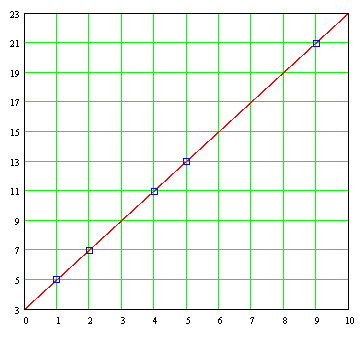

In this graph, the height of each point represents the value of Y for each each pair of values \u200b\u200bX and X
1 2. Representing the points without explicitly show the "highest" points to the horizontal plane Y = 0, making three-dimensional graph like this:
The least squares method used to adjust a set of data to a least squares line can also be extended to obtain a formula of least squares, in which case for two variables the regression equation will the following:
 Y = A + A
 1 X 1 + A 2 X 2
 and often erroneously, this equation is taken as representing a line. However, there is a line, is a surface
 . If we perform a least squares fit on the linear formula with two factors X and X
2, we obtain what is known as a regression
surface, which in this case is a flat surface :
For the data shown above, this surface regression looks like the one shown below: If we get the equations for this least squares plane , we proceed in exactly the same way as we did to get the formulas which evaluate the parameters to obtain the least squares line, that is, we define the vertical distances of each of the ordered pairs of points into this plane of least squares:

By extension, the problems involving more than two variables and

1 X 2
, suppose we start with a relationship between the three variables that can be described by the following formula:
 Y = α
Y = α + ß 1 X
1 + ß 2 X 2
which is a linear formula in the variables
And , X 1 X and 2. Here are three independent parameters α , 1 ß and ß
2. values \u200b\u200band in this line correspond to X 1 = X 1 1 , X 1 2 , X 1 3. .. , X 1 N and 2 X = X 2 1, X 2 2, X 2 3 .. . , X 2 N (we use here the subscript to distinguish each of the two variables X and 1 X 2, and superscript to eventually perform summation over the values \u200b\u200bto each of these variables) are α + ß 1 X 1 1 + ß 2 X 2 1 , α + ß 1 X 1 2 + ß 2 2 X 2 , α + ß 1 X 1 3 + ß 2 X 2 3 ... , Α + ß 1 X 1 N + ß 2 X 2 N , while current values \u200b\u200bare And 1 , Y 2, 3 And ... , And N respectively. Then, as we did on the regression equation based on a single variable, we define the "gap" produced by each trio of experimental data to values \u200b\u200b And i so that the sum of the squares of these distances is: S = (α + ß 1 1 X 1 + ß 2 X 2
1 - Y 1) ² + (α + ß 1 1 X 2 + ß 2 X 2 2 - Y 2) ² + ... + (α + ß 1 X 1 N + ß 2 X 2 N - Y N ) ² from the calculation, S be a minimum when the partial derivatives of S regarding parameters α, ß 1 and 2 ß are equal to zero:
Proceeding as we did when we had two parameters instead of three, this gives us the following set of equations: N α + ß 1 Σ X
1
+ ß  2
2
Σ
 2
2 Σ
X
2
- Σ Y = 0 α Σ X 1 + ß 1 Σ X 1
² + ß
2 Σ X 1 X 2 - Σ X 1 Y = 0 α Σ X 2 + ß 2 Σ X 2
ß ² + 1 Σ X 1 X 2 - X Σ 2 Y = 0 These are the normal equations required to obtain regression in X Y and 1 X 2 . In the calculations, we are three simultaneous equations which are obtained parameters α, ß and
1 ß 2 ² + ß
2 Σ X 1 X 2 - Σ X 1 Y = 0 α Σ X 2 + ß 2 Σ X 2
ß ² + 1 Σ X 1 X 2 - X Σ 2 Y = 0 These are the normal equations required to obtain regression in X Y and 1 X 2 . In the calculations, we are three simultaneous equations which are obtained parameters α, ß and
. There is a reason why these equations are called normal equations. If we represent the data set for the variable X 1 as a vector X 1 and data set for the variable X 2 as another vector X
2
, considering that these vectors are independent of each other (using a term from linear algebra, linearly independent, which means they are not a simple multiple of each other physically pointing in the same direction) then we can put these vectors in a plane. On the other hand, we consider the sum of squared differences D i used in the derivation of normal equations as well as the magnitude of a vector D i , recalling that the square length of a vector is equal to the sum of the squares of its elements ( an extended Pythagorean theorem dimensions). This makes the principle of "best fit" is equivalent to find one difference vector D i corresponding to the shortest possible distance to the plane formed by vectors X 1 X and 2 . And the shortest distance possible is a vector perpendicular or normal vector : the plane defined by vectors X and 1 X 2 (or rather, the plane formed by the linear combination of vectors ß 1 X
+  1 ß 2
1 ß 2
 1 ß 2
1 ß 2 X2). Although we can repeat here the formulas that correspond to the case of two variables X and 1 X 2 , having understood what a "flat of square Mimin "we can use one of many commercially available computer programs or online. The personal page of Professor Victor Miguel Ponce quoted above gives us the means to carry out a" least-squares fit "when it comes to case of two variables X and 1 X 2 , accessible at the following address: http://ponce.sdsu.edu/onlineregression13.php
PROBLEM: Getting the formula plane that best fits the representation of the following data set: These data, represented in three dimensions, are the following aspect:
For this data set, the formula that corresponds to the surface regression is:
Y =  α + ß 1 X
 α + ß 1 X
 1
 + ß 2 X
 2
Y = 9.305829 + 0.787255 X1 - X2 0.04411 Next we have an animated graphic of multiple linear regression and X1 X 2 represented by the formula:
Y = -2
+ 2 X1 X2
where
where
X1 and X2 are varied from -10 to +10 and dimensional graph is rotated around the axis turning And, why this kind of graphs are known under the name "spin plot" (requires enlarge to see the animated action):
The modeling that we conducted can be extended to three variables, four variables, etc., and we can obtain a regression equation Multiple linear:
Y = ß 0 + ß 1 X
1  + ß2
+ ß2
 + ß2
+ ß2 X
2
+ ß3 X 3 + ß 4 X 4 + ß 5 X 5 + ... + ß N X N Unfortunately, for more than two variables is not possible to make a multi-dimensional plotting, and instead of relying on our intuition Geometric have to trust our intuition mathematics. After some practice, we can abandon our reliance on graphical representations extending what we learned into a multi-dimensional world but we can not able to visualize what is happening, giving the crucial step of generalization or abstraction that allows us to dispense with Particulars and still be able to continue working as if nothing had happened. One important thing we have not mentioned yet is that for the case of two variables (as well as more than three variables), we have not taken into account the possible effects of interaction that may exist between the independent variables. These interaction effects, which occur with some frequency in the field of practical applications can be modeled easier if with a formula like this:
Y = ß 0 + ß
Y = ß 0 + ß
1 X 1
+ ß 2 X
2
+ ß 12 X 1 X 2 When no any interaction between variables, the parameter ß 12 shown in this formula is zero . But if there is some kind of interaction, depending on the magnitude of the parameter ß 12 with respect to the other parameters 0
ß, ß
ß, ß
and 1 ß 2 this interaction could be of such magnitude could even nullify the importance of the variable terms ß 1 X 1 and ß 2 X 2 . This issue alone is large enough to require to be dealt with separately in another section of this work.
Subscribe to:
Posts (Atom)