The experimental data fitting non-linear formula, to be obvious that the data can not be adjusted or a least squares line or a polynomial of higher degree, usually requires a mathematical model nonlinear possessing certain characteristics that can maybe even be anticipated theoretically. Take for example the following set of experimental data:
Wednesday, March 26, 2008
density data seem to cluster around something like a logarithmic curve  form y = a + ln
 Obtaining normal equations to perform modeling with non-polynomial equations is similar to the polynomial case. The general equation of three terms:
Y = A + Bf ( X ) + Cg (X )
g (
X) are functions of any variable X
X) + Cg (X ) - And Raising squared residuals and adding, after taking that the partial derivatives with respect to the three parameters
A
,
AΣf ( X ) BΣ + [f
(
x
= ln (
Ae-Bx
A
)
expressed in absolute degrees (Kelvin):
The experience has also confirmed that a formula which can be adjusted very well these experimental data is as follows:
determine the values \u200b\u200bof the constants
A
Using the matrix method, we linearize the problem by making the values \u200b\u200bin what will be the third column of data equal to 1 / T ². We are first row vector with the values \u200b\u200bof p
C
] After that, the data matrix is \u200b\u200bas follows :
Again, we repeat the calculations own matrix method forming the coefficient matrix
:
V = Y ∙ X
to obtain the solution vector
T ∙ V
which gives us the coefficients:
C
x . Estimate the value of the concentration of bacteria when the time is 7 hours. Performing the same steps as those shown in the above problems, the least-squares exponential curve turns out to be:
C = (32.14) (1,427)
when time has elapsed T = 7 hours is, according to this formula: And
= (32.14) (1,427)
7
, stepping out of the range of measured values \u200b\u200bto extend its reach beyond the maximum range covered by the data that generated the curve. This is ultimately one of the main purposes of the curves of least squares: allow researchers to make a quantitative prediction that otherwise would be very subjective and prone to error. Anyway, the smart researcher is not limited to a single mathematical model, and does everything possible to try other models if you have additional factors that need to be taken into account for a better "fit" of data. The graph of the formula obtained, superimposed on the discrete experimental data from which it was generated, is as follows:
: Given the following data pairs (X
i
):
(1, 5.65)
(2, 27.32) (3, 66.7) (4, 98.2) (5, 159.5) (6, 246.3) (7, 325.7) make a least-squares fit of data to an exponential curve of the type Y = ax b . We can carry out calculations using the matrix method as done in previous problems, but will take advantage of the availability of a calculator made available to academic communities around the world by Professor Victor Miguel Ponce of San Diego State University to conduct a set of data to a least-squares exponential curve in precisely the form Y = ax
Y = X 6,104 2,056
Figure original discrete data superimposed on the exponential curve generated by these data is as follows:
adjustment appears to be a good fit, with some discrete points located slightly off the curve.
to
PROBLEM: After an experiment carried out with great care trying to get the most accurate results possible, we obtained the following results: X 1 = 1, Y = 1.81 1 X 2 = 2, Y = 0.75 2 3
X = 3, Y = 0.33
3 4 X = 4, Y = 0,146
4
The graph of this curve with discrete data that generated the formula put in the same graph shows look like :
The negative exponent of 2.02 in the formula seems to have a value very close to integer 2. If we assume that behind this number is a natural law, this number could very well be the integer 2, which has an immediate impact, because according to the algebra: X
2,410
parameter appears to be a simple proportionality constant k
We should be little doubt that the experiment was an experiment in something whose effect is changing
exponential decay (exponential decay) when speed in the fall of some is directly proportional to the amount the balance. To model an exponential decay, we use a formula like this:
Assuming for the sake of simplicity, that C = 1, determine the parameters A and B that are able to adjust the formula for exponential decay to the next set of data:
- tabla_valores_decaimiento_exponencial.png -
-X is a non-linear formula. However, we linearized taking logarithms of both sides of the equation:
]
log [Y (x)] = log (A) + log [B-X
log [Y (X)] = log (A)-xlog (B)
log (8.2 ) ... log (1.19) __ log (0.57)] then form the data matrix X . The first column must contain all ones, which is representative of each of the values \u200b\u200bof X to the power zero. The second column should be formed with the negative of each of the respective values \u200b\u200bof X
:
S = (X T ∙ X) -1
turns out to be:
= 10 = 36,392 1,561
set formula with the numerical data of the experiment is then: Y ( X)
= 36,392 (2,761
should make us suspect that our model parameter
B is actually equal to the number and . This can lead us to refine our formula a little trying to do an adjustment of data for the following model:
Y (X) = Ae-X
In this case, the modeling is much simpler, since we only need to seek a single parameter instead of two. And in this case, to carry out the linearization of the model, we can take advantage of the fact that the exponentiated number is the number and using natural logarithms logarithms instead of base 10, so we can get a closer fit to the "reality" as predicted by a theoretical model accurate.
 ), which can show The following examples
  Obtaining normal equations to perform modeling with non-polynomial equations is similar to the polynomial case. The general equation of three terms:
 Y = A + Bf ( X ) + Cg (X )
where  f (X
f (X
) and
 f (X
f (X ) and
g (
X) are functions of any variable X
. Like as was done since we got the normal equations for least squares line, we define the distances (Waste) as d = A + Bf
(X) + Cg (X ) - And Raising squared residuals and adding, after taking that the partial derivatives with respect to the three parameters
A
,
B and C , we obtain the normal equations: BΣf AN + (X ) CΣg + (X )
= ΣY
= ΣY
AΣf ( X ) BΣ + [f
(
x
) ] ² + CΣf ( x ) g (x ) = Σf (
X
) And AΣg ( X ) + BΣf ( x ) g (X ) CΣ + [g ( X ) ] ² = Σg (
X
) And This is the justification for extending the general matrix method for any type of equation can be linearized. The most immediate way to extend the coverage of the method of least squares to use models non-linear mathematical fit to experimental data to non-linear formula is linearized formula, which often can perform basic mathematical procedures. By way of example, the following non-linear formula: y = Ae-Bx can linearize taking natural logarithms of both sides, which gives: ln (
and
) X
) And AΣg ( X ) + BΣf ( x ) g (X ) CΣ + [g ( X ) ] ² = Σg (
X
) And This is the justification for extending the general matrix method for any type of equation can be linearized. The most immediate way to extend the coverage of the method of least squares to use models non-linear mathematical fit to experimental data to non-linear formula is linearized formula, which often can perform basic mathematical procedures. By way of example, the following non-linear formula: y = Ae-Bx can linearize taking natural logarithms of both sides, which gives: ln (
and
= ln (
Ae-Bx
) ln ( and )
= ln (A
)
+ ln (e -Bx) ln ( and ) = ln ( A ) - Bx which plotted on logarithmic paper gives us a straight line. Without going into too much detail, it may come as good news for many to know that previewed the matrix method can also be used to carry out data adjustment formulas for which there seems to be a simple solution under method of least squares. This can be seen better with the solution of several problems that demonstrate the extent of matrix method to model data with non-linear formulas. PROBLEM : has been experimentally found that the heat capacity of graphite depends on how it documents the following table of data which provides the heat capacity C p (subscript p
indicates that the measurements were carried out at constant pressure, or "outdoor") obtained for various values \u200b\u200bof temperature T
indicates that the measurements were carried out at constant pressure, or "outdoor") obtained for various values \u200b\u200bof temperature T
expressed in absolute degrees (Kelvin):
The experience has also confirmed that a formula which can be adjusted very well these experimental data is as follows:
determine the values \u200b\u200bof the constants
A
,  B and C
to the formula provided.
 B and C
 to the formula provided.
Using the matrix method, we linearize the problem by making the values \u200b\u200bin what will be the third column of data equal to 1 / T ². We are first row vector with the values \u200b\u200bof p
C
: 
Y = [
2.08 2.85 3.50 4.03 4.43 4.75 4.98 5.14 5.27 5.42 
Y = [
] After that, the data matrix is \u200b\u200bas follows :
Again, we repeat the calculations own matrix method forming the coefficient matrix
:
K = X T X ∙
and  constant vector:
 constant vector:
 V = Y ∙ X
to obtain the solution vector
: S = K -1
T ∙ V
which gives us the coefficients:
A = 3.37 B = 0.00191 C =
-177097  thus the "least squares curve is:
 C
p = 3.37 + 0.00191T - 177097 / T ²
The curve superimposed on the original experimental data is as follows:
The curve superimposed on the original experimental data is as follows:
PROBLEM: The water vapor pressure is directly related to temperature. Experimentally obtained with measurements carried out in a laboratory pressure measured in Torr, corresponds to the temperature measured in degrees Celsius, according to the values \u200b\u200blisted in the following table:
After taking a look at various curves available, is that a mathematical model that could describe this behavior is as follows : 
where the temperature is expressed not in degrees Celsius, but in degrees Kelvin (for which you have to convert degrees Celsius to Kelvin by adding 273.15) and where A and B are parameters to be estimated using a "least-squares fit" according to the data obtained experimentally based on the table. Get
first with the nine values \u200b\u200bof pressure P
the row vector we have been calling And
(note that we are taking the natural logarithm of each value, to correspond with the variable that is set on the left side of the formula):
 Y = [ ln (17,535)
_ ln (31,824)
_ ln (55,324) ... ln (760.0) ] after which assemble the data matrix:
We are now with the help of a computer package for handling matrices form the coefficient matrix
V = Y ∙ X
after which we evaluate the solution vector
T ∙ V
getting:
Once the formula, we can plot the curve represents the best fit to the data, superimposed on the discrete data which was obtained. Although we can draw the graph using a logarithmic vertical axis
We can see that experimental data fit the discrete formula is quite good, we could say almost ideal.
This equation is known as the
Clausius-Clapeyron
PROBLEM:
g, expressed in electron-volts (eV) can be determined from the following formula:
1 / ρ = σ
= Ae
- (Eg/2kT) where
ρ is the resistivity expressed in ohms,
T is absolute temperature (degrees Kelvin). The following experimental data were obtained from an intrinsic semiconductor: Linearized first natural formula Logan taking on both sides of it, and carried out after this a "minimal adjustment square "on the experimental data obtained E g for this semiconductor. First take out the linearization taking natural logarithms of both sides of the formula:

applying numerical values, this is already essentially the equation of a line, where Eg/2kT
is the slope of the line. For this problem we will carry out some modifications that will allow us to lighten the execution of the steps involved the matrix method.'ll start with the row vector normally would write after taking natural logarithms of each of the values \u200b\u200bof R , writing now as a column vector :
 There is no objection to what we just did
long as we take the transpose of And
when do the math.
Then we can define the data matrix. It is therefore important to note that you must convert to degrees Celsius (or degrees Celsius) to Kelvin (or absolute degrees) each of the temperatures given in the table of experimental values \u200b\u200b(this is a necessary step in solving many problems of this type, as in formulas Theoretical models of many scientific references to temperatures in degrees Kelvin, not degrees Celsius), which is necessary to add value at each temperature 273.15 under the formula:
K = ° C + 273.15
Using
Now, instead of using three different array formulas as they were doing in the above problems, we may be more comfortable use one. We can obtain as follows:
S = (X
) ∙ (Y ∙ X) T
T ∙ X) T
Using now the property of the transposed
we only condensed formula:
S = (X
directly Putting the data matrix and vector data (this is where the researcher can see the convenience and benefits of using a scientific software package for handling arrays), we obtain the following solution in the form of a column vector:
 E
E
g
= 2 (8.61 • 10 5
Make a least-squares fit of data to an exponential curve of the type Y = ab

where the temperature is expressed not in degrees Celsius, but in degrees Kelvin (for which you have to convert degrees Celsius to Kelvin by adding 273.15) and where A and B are parameters to be estimated using a "least-squares fit" according to the data obtained experimentally based on the table. Get
A and B  . We set
 . We set
 first with the nine values \u200b\u200bof pressure P
the row vector we have been calling And
(note that we are taking the natural logarithm of each value, to correspond with the variable that is set on the left side of the formula):
 Y = [ ln (17,535)
 _ ln (55,324) ... ln (760.0) ] after which assemble the data matrix:
We are now with the help of a computer package for handling matrices form the coefficient matrix
: K = X T X ∙
and constant vector  :
:
 :
: V = Y ∙ X
after which we evaluate the solution vector
S :
S = K -1
S = K -1
T ∙ V
getting:
This solution vector The higher value is the numerical coefficient A and the lower value is the ratio numerical B . On this basis, the equation "best fit" according to the criterion of least squares to the data given is: ln P = 20,459 to 5152 / T
Once the formula, we can plot the curve represents the best fit to the data, superimposed on the discrete data which was obtained. Although we can draw the graph using a logarithmic vertical axis
(the left side of the equation), as used in the past in which the availability of computer programs or even time-shared computer was a luxury almost inaccessible forcing the use of paper semi-logarithmic or logarithmic, today is no longer necessary to resort to such tricks, and we can "clear" formula explicitly putting pressure P as a function of temperature T, thus obtaining the following equation, the following graph of the formula with data discrete superimposed on it: 

We can see that experimental data fit the discrete formula is quite good, we could say almost ideal.
This equation is known as the
Clausius-Clapeyron
. It is important to note that the general pattern of the equation was first obtained theoretically based on arguments based on thermodynamics, and subsequently the model was adjusted carrying out laboratory measurements to determine the parameters and A B
with which the model described and numbered something that can be confirmed in the laboratory. PROBLEM:
The energy band gap of a semiconductor material,  E
E
 E
E g, expressed in electron-volts (eV) can be determined from the following formula:
1 / ρ = σ
= Ae
- (Eg/2kT) where
ρ is the resistivity expressed in ohms,
σ is the electrical conductivity expressed in mhos, k is the Boltzmann constant that can be taken as 8.61x10 -5 and
T is absolute temperature (degrees Kelvin). The following experimental data were obtained from an intrinsic semiconductor: Linearized first natural formula Logan taking on both sides of it, and carried out after this a "minimal adjustment square "on the experimental data obtained E g for this semiconductor. First take out the linearization taking natural logarithms of both sides of the formula:

is the slope of the line. For this problem we will carry out some modifications that will allow us to lighten the execution of the steps involved the matrix method.'ll start with the row vector normally would write after taking natural logarithms of each of the values \u200b\u200bof R , writing now as a column vector :
 There is no objection to what we just did
 long as we take the transpose of
when do the math.
Then we can define the data matrix. It is therefore important to note that you must convert to degrees Celsius (or degrees Celsius) to Kelvin (or absolute degrees) each of the temperatures given in the table of experimental values \u200b\u200b(this is a necessary step in solving many problems of this type, as in formulas Theoretical models of many scientific references to temperatures in degrees Kelvin, not degrees Celsius), which is necessary to add value at each temperature 273.15 under the formula:
K = ° C + 273.15
Using
 Z = 273.15, the data matrix turns out to be:
 Now, instead of using three different array formulas as they were doing in the above problems, we may be more comfortable use one. We can obtain as follows:
S = K -1
T ∙ V S = (X
 ∙ T X) -1
 ) ∙ (Y ∙ X) T
The data row vector And we can get taking the transpose of vector data column And : S = (X ∙ T X) -1 ∙ (Y
T ∙ X) T
Using now the property of the transposed
product of two matrices: (AB) T T = B A T
we only condensed formula:
S = (X
∙ T X) -1 ∙ (X T ∙ Y)
directly Putting the data matrix and vector data (this is where the researcher can see the convenience and benefits of using a scientific software package for handling arrays), we obtain the following solution in the form of a column vector:
Then: - E g / 2kT
= 3483 • 10 3
= 3483 • 10 3
 E
E g
= 2 (8.61 • 10 5
) (3,483 • 10 3 ) E
g = 0.6 electron-volts PROBLEM: A notable example is provided by the exponential growth of bacterial cultures samples. The following table, assume that the number of bacteria per unit volume is given by the variable C after T
hours of culture.
hours of culture.
x . Estimate the value of the concentration of bacteria when the time is 7 hours. Performing the same steps as those shown in the above problems, the least-squares exponential curve turns out to be:
C = (32.14) (1,427)
T 
value Y 
when time has elapsed T = 7 hours is, according to this formula: And
= (32.14) (1,427)
7
And
= 387.27 Note that here it is conducting an extrapolation
= 387.27 Note that here it is conducting an extrapolation
, stepping out of the range of measured values \u200b\u200bto extend its reach beyond the maximum range covered by the data that generated the curve. This is ultimately one of the main purposes of the curves of least squares: allow researchers to make a quantitative prediction that otherwise would be very subjective and prone to error. Anyway, the smart researcher is not limited to a single mathematical model, and does everything possible to try other models if you have additional factors that need to be taken into account for a better "fit" of data. The graph of the formula obtained, superimposed on the discrete experimental data from which it was generated, is as follows:
We can see that the data fit the formula is excellent. There are also many natural phenomena growth of bacteria that can be described by an exponential model as the one just used here.
This problem is representative of problems that can make predictions with phenomena that may play to public health even in cases of an epidemic out of control.
PROBLEM
This problem is representative of problems that can make predictions with phenomena that may play to public health even in cases of an epidemic out of control.
PROBLEM
: Given the following data pairs (X
i
,  And
And
i
 And
And i
):
(1, 5.65)
(2, 27.32) (3, 66.7) (4, 98.2) (5, 159.5) (6, 246.3) (7, 325.7) make a least-squares fit of data to an exponential curve of the type Y = ax b . We can carry out calculations using the matrix method as done in previous problems, but will take advantage of the availability of a calculator made available to academic communities around the world by Professor Victor Miguel Ponce of San Diego State University to conduct a set of data to a least-squares exponential curve in precisely the form Y = ax
b
at the following address :
http://ponce.sdsu.edu/onlineregression12.php
Using the calculator, we obtain as a way of "best fit"
at the following address :
http://ponce.sdsu.edu/onlineregression12.php
Using the calculator, we obtain as a way of "best fit"
Y = X 6,104 2,056
Figure original discrete data superimposed on the exponential curve generated by these data is as follows:
adjustment appears to be a good fit, with some discrete points located slightly off the curve.
This problem is similar to the previous problem except for one important difference: in the previous problem was adjusted to a formula of the form y = ab X , while this problem was adjusted to a formula of the form Y = aX
b
. While the model used in the previous problem intersects the vertical axis at a different point Y = 0 b
to
X = 0, the model used in this issue intersects the vertical axis precisely in Y = 0  to X = 0
, which can be important in some physical applications where the exponential growth starts precisely from the "zero point".
 to X = 0
 , which can be important in some physical applications where the exponential growth starts precisely from the "zero point".
PROBLEM: After an experiment carried out with great care trying to get the most accurate results possible, we obtained the following results: X 1 = 1, Y = 1.81 1 X 2 = 2, Y = 0.75 2 3
X = 3, Y = 0.33
3 4 X = 4, Y = 0,146
4
5 X = 5, And 5 = 0.118 X
6 = 6, Y = 0.05 6 X
7 = 7, Y = 0.037 7
Adjust these experimental data to a Type
Y = aX b . What kind of experiment data seem to be suggesting?
we proceed as we did in the previous problem, where we use the same model. If we do this, we obtain the following formula:
Y = 2,410 X
-2.02
6 = 6, Y = 0.05 6 X
7 = 7, Y = 0.037 7
Adjust these experimental data to a Type
Y = aX b . What kind of experiment data seem to be suggesting?
we proceed as we did in the previous problem, where we use the same model. If we do this, we obtain the following formula:
Y = 2,410 X
-2.02
The graph of this curve with discrete data that generated the formula put in the same graph shows look like :
The negative exponent of 2.02 in the formula seems to have a value very close to integer 2. If we assume that behind this number is a natural law, this number could very well be the integer 2, which has an immediate impact, because according to the algebra: X
= 1 -2 / X ²
2,410
parameter appears to be a simple proportionality constant k
to match the units on both sides of the formula, properly dimensioned. In this case, the formula can be rewritten symbolically as: 
Y = k ∙ (1 / X ²)

Y = k ∙ (1 / X ²)
We should be little doubt that the experiment was an experiment in something whose effect is changing
in inverse proportion to the square of another quantity , an amount that could well be a distance. It is quite possible that this experiment was an experiment to verify the change in inverse proportion to the square of the distance predicted by the law of universal gravitation by Sir Isaac Newton, or an experiment to verify the change in inverse proportion to the square of distance from the force of attraction or repulsion between two electric charges of opposite signs or similar signs predicted by Coulomb's law. It We said in the statement of the problem that the experiment was carried out carefully, and yet several discrete experimental data fell visibly out of the curve does appear to be the curve of "best fit", which tells us that the experiment was carried out under difficult circumstances that required all the skill that the researchers could deploy in the experiment. PROBLEM:
A phenomenon that occurs frequently in nature is the phenomenon related to
A phenomenon that occurs frequently in nature is the phenomenon related to
exponential decay (exponential decay) when speed in the fall of some is directly proportional to the amount the balance. To model an exponential decay, we use a formula like this:
Y (X) = A • B
-CX Assuming for the sake of simplicity, that C = 1, determine the parameters A and B that are able to adjust the formula for exponential decay to the next set of data:
- tabla_valores_decaimiento_exponencial.png -
formula Y (X) = A · B
-X is a non-linear formula. However, we linearized taking logarithms of both sides of the equation:
]

log [Y (x)] = log (A) + log [B-X
]
log [Y (X)] = log (A)-xlog (B)
log [Y (X)] = log (A) - log (B) · X
Using P = log [Y (X)]
, Q = log (A) and R = log (B) , we have a linear relationship on which you can apply least squares adjustment with the help of the matrix method. First assemble a data vector And in which we take the logarithm of each of the values \u200b\u200bof And
:
Y = [log (35) __ log (23) __
log (12.1) __
log (8.2 ) ... log (1.19) __ log (0.57)] then form the data matrix X . The first column must contain all ones, which is representative of each of the values \u200b\u200bof X to the power zero. The second column should be formed with the negative of each of the respective values \u200b\u200bof X
:
This formed, we can directly apply the condensed array formula that will give us the solution vector S :
S = (X T ∙ X) -1
∙ (X 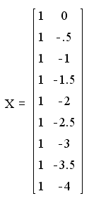
T ∙ Y)

T ∙ Y)
turns out to be:
is important to remember that these values \u200b\u200bcorrespond to the linearized formula on which the logs were taken. values \u200b\u200b A and B are obtained by taking the antilog of the numbers given by the solution matrix, which is equivalent to raising the base (10) to those numbers as exponents
A = 10 = 36,392 1,561
B 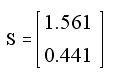
= 10 = 2,761 0,441

= 10 = 2,761 0,441
set formula with the numerical data of the experiment is then: Y ( X)
= 36,392 (2,761
) -X
The graph of this formula with discrete data that generated superimposed on it is:
The graph of this formula with discrete data that generated superimposed on it is:
We can see that the formula is adjusted reasonably well to the discrete data which was generated. If we look at the formula we obtained, we can see that the parameter B which is equal to 2,761 is a number that is very close to the number e = 2.7182, which is not only the base of natural logarithms, but also a number that appears in the solution of many theoretical formulas (exact) coming from the solution of a differential equation simple:
dY / dx =-Y An example of this kind of formulas is that of  radioactive decay exponentially, the basic phenomenon of nuclear physics. The observation that the result we obtained for the parameter B
is very, very close to the number and
 radioactive decay exponentially, the basic phenomenon of nuclear physics. The observation that the result we obtained for the parameter B
 is very, very close to the number and
should make us suspect that our model parameter
B is actually equal to the number and . This can lead us to refine our formula a little trying to do an adjustment of data for the following model:
Y (X) = Ae-X
In this case, the modeling is much simpler, since we only need to seek a single parameter instead of two. And in this case, to carry out the linearization of the model, we can take advantage of the fact that the exponentiated number is the number and using natural logarithms logarithms instead of base 10, so we can get a closer fit to the "reality" as predicted by a theoretical model accurate.
Subscribe to:
Post Comments (Atom)
0 comments:
Post a Comment