
easier adjustment formula data that we can carry out is one in which the data show a linear trend in which the data appear to follow a trend in a straight line when placed on a graph. The first step, before anything, is to translate data into a graph at our disposal to determine if indeed there is any trend (either linear or nonlinear) for grouped data following a certain trend, behind which there is possibly a natural relationship that eventually can be expressed with a simple formula. If the graph of the data from several pairs of measurements of two variable quantities, of which perhaps can be varied at will, this is a as follows:

we can see that there seems to be no correlation between the graphed data. However, if the graph turns out to be one like this:

then it manifests as a tendency. These data, allegedly obtained by experiment, usually to be affected with a random error (occurring at random) denoted by the Greek letter ε (equivalent to the Latin letter "e"). If it were not for this error, possibly all the data fall in a straight line or a smooth, continuous curve of the phenomenon itself is being described by the data. In the last graph, it is tempting to draw "by hand" on the same straight line as close as possible to our data, a straight line like the following:

The problem with a plot "by hand" of the straight line is that different people get different lines according to their own subjective criteria, and possibly no one will have the same line, having no way of knowing which of them is the best. That is why, in order to unify criteria and get the same answer in all cases, we need to use a mathematical approach . This approach gives us the method of least squares , developed by the "prince of mathematics" Carl Friedrich Gauss.
The idea behind the method of least squares is as follows: if on a dataset in a graph that seem to cluster along a trend marked by a straight line is drawn a straight line, then all the different lines that can be drawn we can try to find one which produces "best fit" (in English this is called best fit) of according to some mathematical criterion. This line may be that such that the "average distance" from all points on the graph to the ideal line is the smallest average distance possible. Although the distances of each point to the ideal line can be defined so as to be perpendicular to the line, as shown in the picture below right:

mathematical manipulation of the problem can be greatly simplified if instead of using such distances perpendicular to the ideal use vertical distances as the vertical axis of the graph as shown in the picture above left.
While we could try to use absolute values \u200b\u200b d │ i │ distances of each of the points i to the ideal line (the absolute values \u200b\u200beliminate the presence of negative values \u200b\u200baveraged over the Positive values \u200b\u200bwould end "canceling" We intend to obtain a useful average), the main problem is that the absolute value any variable can not be differentiated mathematically in a conventional manner, not easily lend itself to a mathematical derivation using the usual resources of differential calculus, which is a disadvantage when they go to use the tools of the calculation to obtain the maximum and minimum. That is why we use the sum of the squares distances rather than the absolute values \u200b\u200bof the same, as this allows us to treat these securities, known as residual , as a quantity continuously differentiable. However, this technique has the disadvantage that when used square of the distance those isolated points are very far from the ideal line will have an effect on the setting, something that we should not lose sight of when they appear isolated in the graph data that seem too far from the ideal line and which may be indicative of a mistake in measurement or bad data recorded.
For data that seem to show a linear trend, according to the method of least squares is assumed from the outset the existence of a line "ideal" that provides the best fit (best fit ) known as "least-squares fit (least squares fit ). The equation of this "ideal line" is:
where A and B are the parameters (constant number) to be determined under the criterion of least squares.
Given a number N of pairs of experimental points (X 1 , And 1), (2 X, Y 2), (X 3 , And 3), etc., then for each experimental point corresponding to each value of the independent variable X = X 1 , X 2, X 3 ,..., X N be a calculated value and i = and 1 , and 2, and 3 ... using the straight "ideal", which is:
The difference between real value of Y = Y 1 , Y 2, and 3 ,..., Y N and each value calculated for the corresponding X i using the ideal line gives us the "distance" vertical D i that alienates both values:
Each of these distances D i is known in mathematical statistics as the residual .
straight To find the "ideal", we will use the established procedures of differential calculus for determining the maximum and minimum. A first attempt to lead us to try and find the line that minimizes the sum of the distances
However, this scheme will not serve us much, because the calculations to determine the value of each distance D i some points "real" above the line will and others will be below it, which some of the distances are positive and some negative (possibly distributed in equal parts) thus canceling much of their contributions the construction of the function you want to minimize. This leads us immediately to try to use absolute values \u200b\u200b distances:
3 ² + ... + D N ²
2) ² + (A + BX 3
The solution of these equations gives us the equations required:
AN + B Σ
X -
Σ Y = 0

Σ A X + B
And

A
Σ
X + B
PROBLEM:
Given the following, obtain the line of least squares:

To use the equations required to obtain the line of least squares, it is desirable to accommodate the summation in a table like the one shown below:
From this table of intermediate results we obtain:
(
X ²
)
Σ
X ² -
see that the fit is reasonably good. And, most important, other researchers will get exactly the same result under the criterion of square Mimin such problems. Significantly, the mechanization of the evaluation of these data by columns such as arrangements that were used up getting
Σ
and
X ² Σ XY 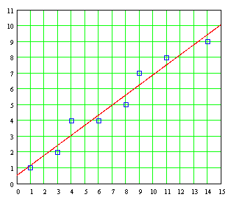 can be done in a "worksheet" as EXCEL.
For a large set of data pairs, other times these calculations used to be tedious and subject to mistakes. Fortunately, with the advent of programmable pocket calculators and computer programs that can now be performed on a desktop computer arithmetic for which only two decades ago required expensive computers and sophisticated software in a scientific programming language such as FORTRAN These calculations can be machined to such an extent that instead of having to use excessive amounts of time in performing the calculations the emphasis today is on and l analysis and interpretation of results
. If, on the basis of experimental data or data obtained from a sample taken from a population we want to estimate the value of a variable Y corresponding to a value of another variable X from the least-squares curve best fits the data, it is customary to call the resulting curve the regression curve of Y in X since And is estimated X . If the curve is a straight line, then call that line the regression line of Y on X . An analysis carried out by the method of least squares is also called regression analysis, and computer programs that can perform calculations are called least-squares regression programs
. If, however, instead of estimating the value of
And
from X value we wish to estimate the value of X from And then we would use a curve regression of X on Y , which involves simply exchanging the variables in the diagram (and in the normal equations) so that X is the dependent variable and And the independent variable, which in turn means replacing the vertical distances D used in the derivation of the least squares line for horizontal distances :
An interesting detail is that, generally, for a given set of data the regression line in X Y and the regression line in X Y two different lines that do not match exactly in a diagram, but in any case are so close to each other that could be confused.
PROBLEM:
a) Get the regression line of Y on X, given Y as the dependent variable and X as independent variable. b)
Get the regression line of X on Y, given X and Y as the dependent variable as independent variable.
a) Considering Y as the dependent variable and X as the independent variable, the equation of the least squares line is Y = A + BX, and the normal equations are: BΣX ΣY = AN +
ΣXY = AΣX + BΣX ² 8A + 56B = 40
56A + 524B = 364
Simultaneous two equations, we get A = 6 / 11 and B = 7 / 11. Then the least squares line is:
Y = 6 / 11 + (7 / 11) X
Y = 0.545 + 0.636 X
b) Considering X as the dependent variable and Y as independent variable, the least squares equation is now X = P + QY, and normal equations are:
sx = PN + QΣY
8P +
X = -0.5 + 1.5Y
For comparative purposes, we can solve this formula to make And depending on X, obtaining:
Y = 0.333 + 0.667 X
We note that the regression lines obtained in (a) and (b)
different. Below is a chart showing the two lines:
An important measure of how well is the "adjustment" of various experimental data to a straight line obtained from the minimum by the method of least squares is the correlation coefficient
. When all the data is located exactly on a straight line, then
correlation coefficient is unity, and as data on a graph will show increasingly dispersed in relation to the line then the correlation coefficient gradually decreases as shown by the following examples:
As a courtesy of Professor Victor Miguel Ponce, professor and researcher at San Diego State University are available to the public on his personal website on the Internet several programs to machine calculations required to "adjust" data set with a linear trend line of "least squares". The page that provides all programs is:
To use the above program, we introduce first the size of the array (array ), or the amount of data pairs, after which we introduce the values \u200b\u200b
paired data in an orderly manner starting first with the values \u200b\u200bseparated by commas, followed by the values \u200b\u200bof x, also separated by commas. Done, press "Calculate" at the bottom of the page, which we obtain the values \u200b\u200bα
, the correlation coefficient
r
The standard error
estimation and dispersions (standard deviations) σ
x and σ and data x i and data and i . As an example of using this program, we obtain the least squares line for the following pairs of data: x (1) = 1 and (1) = 5 x (2) = 2, and ( 2) = 7 x (3) = 4, and (3) = 11 x (4) = 5, and (4) = 13 x (5) = 9, and (5) = 21 De Under this program, least squares line is: Y = 3 + 2X And the correlation coefficient r is
= 1.0, while the standard error of the estimate is zero, which as we shall see later tells us that
all pairs of data are part of the line of least squares
. If we plot the least squares line and plotted on it the data pairs (x
i
,
and
which confirms that the mathematical criterion that we used to get the line of least squares, we have defined the correlation index r are correct, we have defined the standard error of the estimate is correct . far we have considered a "least-squares fit" associated with a line that might be called "ideal" from a mathematical point of view, where we have an independent variable (cause) that produces an effect on some dependent variable (effect) . But it may be the case we have a situation in which some variable values \u200b\u200btake will be dependent on not one but two or more factors. In this case, if the individual unit because each of the factors, keeping the other constant, is a linear dependence, we can extend the method of least squares to cover this situation as we did when there was only one variable independent. This is known as a multiple linear regression . For two variables X and X 1 2, this dependence is represented as Y = f (X
1, X 2
In this graph, the height of each point represents the value of Y for each each pair of values \u200b\u200bX and X
1 2. Representing the points without explicitly show the "highest" points to the horizontal plane Y = 0, making three-dimensional graph like this:
The least squares method used to adjust a set of data to a least squares line can also be extended to obtain a formula of least squares, in which case for two variables the regression equation will the following:
1 X 1 + A 2 X 2
 and often erroneously, this equation is taken as representing a line. However, there is a line, is a surface
. If we perform a least squares fit on the linear formula with two factors X and X 1
2, we obtain what is known as a regression
If we get the equations for this least squares plane , we proceed in exactly the same way as we did to get the formulas which evaluate the parameters to obtain the least squares line, that is, we define the vertical distances of each of the ordered pairs of points into this plane of least squares:

By extension, the problems involving more than two variables and
1 X 2
, suppose we start with a relationship between the three variables that can be described by the following formula:
 Y = α
Y = α
+ ß 1 X
1 + ß 2 X 2
which is a linear formula in the variables
2. values \u200b\u200band in this line correspond to X 1 = X 1 1 , X 1 2 , X 1 3. .. , X 1 N and 2 X = X 2 1, X 2 2, X 2 3 .. . , X 2 N (we use here the subscript to distinguish each of the two variables X and 1 X 2, and superscript to eventually perform summation over the values \u200b\u200bto each of these variables) are α + ß 1 X 1 1 + ß 2 X 2 1 , α + ß 1 X 1 2 + ß 2 2 X 2 , α + ß 1 X 1 3 + ß 2 X 2 3 ... , Α + ß 1 X 1 N + ß 2 X 2 N , while current values \u200b\u200bare And 1 , Y 2, 3 And ... , And N respectively. Then, as we did on the regression equation based on a single variable, we define the "gap" produced by each trio of experimental data to values \u200b\u200b And i so that the sum of the squares of these distances is: S = (α + ß 1 1 X 1 + ß 2 X 2
Proceeding as we did when we had two parameters instead of three, this gives us the following set of equations: N α + ß 1 Σ X
1
X
2
. There is a reason why these equations are called normal equations. If we represent the data set for the variable X 1 as a vector X 1 and data set for the variable X 2 as another vector X
2
, considering that these vectors are independent of each other (using a term from linear algebra, linearly independent, which means they are not a simple multiple of each other physically pointing in the same direction) then we can put these vectors in a plane. On the other hand, we consider the sum of squared differences D i used in the derivation of normal equations as well as the magnitude of a vector D i , recalling that the square length of a vector is equal to the sum of the squares of its elements ( an extended Pythagorean theorem dimensions). This makes the principle of "best fit" is equivalent to find one difference vector D i corresponding to the shortest possible distance to the plane formed by vectors X 1 X and 2 . And the shortest distance possible is a vector perpendicular or normal vector : the plane defined by vectors X and 1 X 2 (or rather, the plane formed by the linear combination of vectors ß 1 X
X2). Although we can repeat here the formulas that correspond to the case of two variables X and 1 X 2 , having understood what a "flat of square Mimin "we can use one of many commercially available computer programs or online. The personal page of Professor Victor Miguel Ponce quoted above gives us the means to carry out a" least-squares fit "when it comes to case of two variables X and 1 X 2 , accessible at the following address: http://ponce.sdsu.edu/onlineregression13.php
PROBLEM: Getting the formula plane that best fits the representation of the following data set: These data, represented in three dimensions, are the following aspect:
For this data set, the formula that corresponds to the surface regression is:
1
2
Y = -2
X1 and X2 are varied from -10 to +10 and dimensional graph is rotated around the axis turning And, why this kind of graphs are known under the name "spin plot" (requires enlarge to see the animated action):
Y = ß 0 + ß 1 X
X
2
1 X 1
+ ß 2 X
2
and 1 ß 2 this interaction could be of such magnitude could even nullify the importance of the variable terms ß 1 X 1 and ß 2 X 2 . This issue alone is large enough to require to be dealt with separately in another section of this work.
The idea behind the method of least squares is as follows: if on a dataset in a graph that seem to cluster along a trend marked by a straight line is drawn a straight line, then all the different lines that can be drawn we can try to find one which produces "best fit" (in English this is called best fit) of according to some mathematical criterion. This line may be that such that the "average distance" from all points on the graph to the ideal line is the smallest average distance possible. Although the distances of each point to the ideal line can be defined so as to be perpendicular to the line, as shown in the picture below right:

mathematical manipulation of the problem can be greatly simplified if instead of using such distances perpendicular to the ideal use vertical distances as the vertical axis of the graph as shown in the picture above left.
While we could try to use absolute values \u200b\u200b d │ i │ distances of each of the points i to the ideal line (the absolute values \u200b\u200beliminate the presence of negative values \u200b\u200baveraged over the Positive values \u200b\u200bwould end "canceling" We intend to obtain a useful average), the main problem is that the absolute value any variable can not be differentiated mathematically in a conventional manner, not easily lend itself to a mathematical derivation using the usual resources of differential calculus, which is a disadvantage when they go to use the tools of the calculation to obtain the maximum and minimum. That is why we use the sum of the squares distances rather than the absolute values \u200b\u200bof the same, as this allows us to treat these securities, known as residual , as a quantity continuously differentiable. However, this technique has the disadvantage that when used square of the distance those isolated points are very far from the ideal line will have an effect on the setting, something that we should not lose sight of when they appear isolated in the graph data that seem too far from the ideal line and which may be indicative of a mistake in measurement or bad data recorded.
For data that seem to show a linear trend, according to the method of least squares is assumed from the outset the existence of a line "ideal" that provides the best fit (best fit ) known as "least-squares fit (least squares fit ). The equation of this "ideal line" is:
Y = A + BX
where A and B are the parameters (constant number) to be determined under the criterion of least squares.
Given a number N of pairs of experimental points (X 1 , And 1), (2 X, Y 2), (X 3 , And 3), etc., then for each experimental point corresponding to each value of the independent variable X = X 1 , X 2, X 3 ,..., X N be a calculated value and i = and 1 , and 2, and 3 ... using the straight "ideal", which is:
and 1 = A + BX 1
and 2 = A + BX 2
and 3 = A + BX 3
.
.
.
and N = A + BX N
and 2 = A + BX 2
and 3 = A + BX 3
.
.
.
and N = A + BX N
The difference between real value of Y = Y 1 , Y 2, and 3 ,..., Y N and each value calculated for the corresponding X i using the ideal line gives us the "distance" vertical D i that alienates both values:
D 1 = A + BX 1 - Y 1
2 D = A + BX 2 - And 2
D 3 = A + BX 3 - Y 3
.
.
.
D N = A + BX N - Y N
2 D = A + BX 2 - And 2
D 3 = A + BX 3 - Y 3
.
.
.
D N = A + BX N - Y N
Each of these distances D i is known in mathematical statistics as the residual .
straight To find the "ideal", we will use the established procedures of differential calculus for determining the maximum and minimum. A first attempt to lead us to try and find the line that minimizes the sum of the distances
S = D 1 + D + D 2 3 + ... D + N
However, this scheme will not serve us much, because the calculations to determine the value of each distance D i some points "real" above the line will and others will be below it, which some of the distances are positive and some negative (possibly distributed in equal parts) thus canceling much of their contributions the construction of the function you want to minimize. This leads us immediately to try to use absolute values \u200b\u200b distances:
S = another scheme in which we also add the distances D i but without the problem of mutual cancellation of terms having positive and negative terms. The strategy is to use squares of the distances: S = D 1 D ² + 2 ² + D
3 ² + ... + D N ²
With this definition, the general term we want to minimize is given by: S = (A + BX 1 And 1 ) ² + (A + BX 2 And
2) ² + (A + BX 3
And 3) ² + ... + (A + BX N-Y N ) ² The unknowns of the line we are looking for are ideal parameters and A B . With respect to these two questions is how we must carry out the minimization of S . If it were a single parameter, a sufficient ordinary differentiation. But since there are two parameters, we must carry out two separate distinctions derived using partial in which we differentiate with respect to a parameter keeping the other constant. from the calculation, S be a minimum when the partial derivatives with respect to A and B are zero. These partial derivatives are:
The solution of these equations gives us the equations required:
AN + B Σ
X -
Σ Y = 0

Σ A X + B
Σ X ² - Σ XY = 0
where we are using the following simplified symbolic notation:
where we are using the following simplified symbolic notation:
The two equations we can rearrange as follows: AN + B Σ X =
Σ And

A
Σ
X + B
Σ X ² = Σ XY
taking with it two equations linear which can be solved as simultaneous equations either directly or through the method of Cramer (determinants), thus obtaining the following formulas:
taking with it two equations linear which can be solved as simultaneous equations either directly or through the method of Cramer (determinants), thus obtaining the following formulas:
Thus, the substitution of data in the two formulas give us the values \u200b\u200bof the parameters and A B we are looking for and the "ideal line, the line provides the best fit of all that we can draw on the criteria we defined. Since we are minimizing a function that minimizes the sum of the squares of the distances (residuals), this method as mentioned above is known universally as the method of least square.
PROBLEM:
Given the following, obtain the line of least squares:

To use the equations required to obtain the line of least squares, it is desirable to accommodate the summation in a table like the one shown below:
From this table of intermediate results we obtain:
(
Σ  And
And
) (
Σ  And
And ) (
X ²
)
- (Σ 
X) ( Σ 
XY) = (40) (524) - (56) (364) = 6 N Σ XY - (X Σ) (Σ And ) = (8) (364) - (56) (40) = 7 N
Σ
X ² - ( Σ X ) ² = (8) (524) - (56 ) ² = 11 And using the above formulas obtained:
A = [
( AND Σ) (Σ X ² ) - ( Σ
X) (XY Σ
X ² - ( Σ X ) ² = (8) (524) - (56 ) ² = 11 And using the above formulas obtained:
A = [
( AND Σ) (Σ X ² ) - ( Σ
Σ
) ] / [N Σ X ² - (Σ X ) ²] = 6 / 11 A = .545 B = [N Σ XY - ( Σ X ) ( Σ
And
) ] / [N
Σ
And
) ] / [N
Σ
X ² -
( Σ X ) ²] = 7 / 11 B = .636 The least squares line is then: Y = A + BX Y = 0.545 + 0.636 X The graph of this straight line superimposed on the individual point pairs is:
We see that the fit is reasonably good. And, most important, other researchers will get exactly the same result under the criterion of square Mimin such problems. Significantly, the mechanization of the evaluation of these data by columns such as arrangements that were used up getting
Σ
X, Y
Σ , Σ
Σ , Σ
and
X ² Σ XY
 can be done in a "worksheet" as EXCEL.
 For a large set of data pairs, other times these calculations used to be tedious and subject to mistakes. Fortunately, with the advent of programmable pocket calculators and computer programs that can now be performed on a desktop computer arithmetic for which only two decades ago required expensive computers and sophisticated software in a scientific programming language such as FORTRAN These calculations can be machined to such an extent that instead of having to use excessive amounts of time in performing the calculations the emphasis today is on and
. If, on the basis of experimental data or data obtained from a sample taken from a population we want to estimate the value of a variable Y corresponding to a value of another variable X from the least-squares curve best fits the data, it is customary to call the resulting curve the regression curve of Y in X since And is estimated X . If the curve is a straight line, then call that line the regression line of Y on X . An analysis carried out by the method of least squares is also called regression analysis, and computer programs that can perform calculations are called least-squares regression programs
. If, however, instead of estimating the value of
And
from X value we wish to estimate the value of X from And then we would use a curve regression of X on Y , which involves simply exchanging the variables in the diagram (and in the normal equations) so that X is the dependent variable and And the independent variable, which in turn means replacing the vertical distances D used in the derivation of the least squares line for horizontal distances :
An interesting detail is that, generally, for a given set of data the regression line in X Y and the regression line in X Y two different lines that do not match exactly in a diagram, but in any case are so close to each other that could be confused.
PROBLEM:
Given the following data set: 

a) Get the regression line of Y on X, given Y as the dependent variable and X as independent variable. b)
Get the regression line of X on Y, given X and Y as the dependent variable as independent variable.
a) Considering Y as the dependent variable and X as the independent variable, the equation of the least squares line is Y = A + BX, and the normal equations are: BΣX ΣY = AN +
ΣXY = AΣX + BΣX ² 8A + 56B = 40
 Carrying out the summation, the normal equations become:
 56A + 524B = 364
Simultaneous two equations, we get A = 6 / 11 and B = 7 / 11. Then the least squares line is:
Y = 6 / 11 + (7 / 11) X
Y = 0.545 + 0.636 X
b) Considering X as the dependent variable and Y as independent variable, the least squares equation is now X = P + QY, and normal equations are:
sx = PN + QΣY
ΣXY = PΣY + QΣY ²
Carrying out the summation, the normal equations become:
Carrying out the summation, the normal equations become:
8P +
40Q = 56 = 364 40P + 256Q Simultaneous
both equations, we obtain P =- 1 / 2 and Q = 3 / 2. Then the least squares line is:
X = -1 / 2 + (3 / 2) Y both equations, we obtain P =- 1 / 2 and Q = 3 / 2. Then the least squares line is:
X = -0.5 + 1.5Y
For comparative purposes, we can solve this formula to make And depending on X, obtaining:
Y = 0.333 + 0.667 X
We note that the regression lines obtained in (a) and (b)
different. Below is a chart showing the two lines:
An important measure of how well is the "adjustment" of various experimental data to a straight line obtained from the minimum by the method of least squares is the correlation coefficient
correlation coefficient is unity, and as data on a graph will show increasingly dispersed in relation to the line then the correlation coefficient gradually decreases as shown by the following examples:
As a courtesy of Professor Victor Miguel Ponce, professor and researcher at San Diego State University are available to the public on his personal website on the Internet several programs to machine calculations required to "adjust" data set with a linear trend line of "least squares". The page that provides all programs is:
http://ponce.sdsu.edu/online_calc.php  under the heading of "Regression." The page that we want to obtain a data fit a straight line is located at:
Http://ponce.sdsu.edu/onlineregression11.php
 under the heading of "Regression." The page that we want to obtain a data fit a straight line is located at:
 Http://ponce.sdsu.edu/onlineregression11.php
To use the above program, we introduce first the size of the array (array ), or the amount of data pairs, after which we introduce the values \u200b\u200b
paired data in an orderly manner starting first with the values \u200b\u200bseparated by commas, followed by the values \u200b\u200bof x, also separated by commas. Done, press "Calculate" at the bottom of the page, which we obtain the values \u200b\u200bα
and ß  for least squares line and
= α + ßx
 for least squares line and
 = α + ßx
, the correlation coefficient
r
The standard error
estimation and dispersions (standard deviations) σ
x and σ and data x i and data and i . As an example of using this program, we obtain the least squares line for the following pairs of data: x (1) = 1 and (1) = 5 x (2) = 2, and ( 2) = 7 x (3) = 4, and (3) = 11 x (4) = 5, and (4) = 13 x (5) = 9, and (5) = 21 De Under this program, least squares line is: Y = 3 + 2X And the correlation coefficient r is
= 1.0, while the standard error of the estimate is zero, which as we shall see later tells us that
all pairs of data are part of the line of least squares
. If we plot the least squares line and plotted on it the data pairs (x
i
,
and
i), we find that indeed all data is aligned directly over a line:
which confirms that the mathematical criterion that we used to get the line of least squares, we have defined the correlation index r are correct, we have defined the standard error of the estimate is correct . far we have considered a "least-squares fit" associated with a line that might be called "ideal" from a mathematical point of view, where we have an independent variable (cause) that produces an effect on some dependent variable (effect) . But it may be the case we have a situation in which some variable values \u200b\u200btake will be dependent on not one but two or more factors. In this case, if the individual unit because each of the factors, keeping the other constant, is a linear dependence, we can extend the method of least squares to cover this situation as we did when there was only one variable independent. This is known as a multiple linear regression . For two variables X and X 1 2, this dependence is represented as Y = f (X
1, X 2
). If you have a set of experimental data for a situation like this, the graphic data must be carried out in three dimensions, and its appearance is as follows: 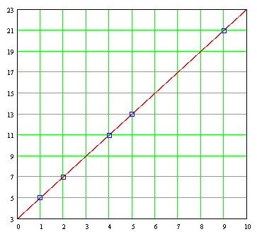

In this graph, the height of each point represents the value of Y for each each pair of values \u200b\u200bX and X
1 2. Representing the points without explicitly show the "highest" points to the horizontal plane Y = 0, making three-dimensional graph like this:
The least squares method used to adjust a set of data to a least squares line can also be extended to obtain a formula of least squares, in which case for two variables the regression equation will the following:
 Y = A + A
 1 X 1 + A 2 X 2
 and often erroneously, this equation is taken as representing a line. However, there is a line, is a surface
 . If we perform a least squares fit on the linear formula with two factors X and X
2, we obtain what is known as a regression
surface, which in this case is a flat surface :
For the data shown above, this surface regression looks like the one shown below: If we get the equations for this least squares plane , we proceed in exactly the same way as we did to get the formulas which evaluate the parameters to obtain the least squares line, that is, we define the vertical distances of each of the ordered pairs of points into this plane of least squares:

By extension, the problems involving more than two variables and

1 X 2
, suppose we start with a relationship between the three variables that can be described by the following formula:
 Y = α
Y = α + ß 1 X
1 + ß 2 X 2
which is a linear formula in the variables
And , X 1 X and 2. Here are three independent parameters α , 1 ß and ß
2. values \u200b\u200band in this line correspond to X 1 = X 1 1 , X 1 2 , X 1 3. .. , X 1 N and 2 X = X 2 1, X 2 2, X 2 3 .. . , X 2 N (we use here the subscript to distinguish each of the two variables X and 1 X 2, and superscript to eventually perform summation over the values \u200b\u200bto each of these variables) are α + ß 1 X 1 1 + ß 2 X 2 1 , α + ß 1 X 1 2 + ß 2 2 X 2 , α + ß 1 X 1 3 + ß 2 X 2 3 ... , Α + ß 1 X 1 N + ß 2 X 2 N , while current values \u200b\u200bare And 1 , Y 2, 3 And ... , And N respectively. Then, as we did on the regression equation based on a single variable, we define the "gap" produced by each trio of experimental data to values \u200b\u200b And i so that the sum of the squares of these distances is: S = (α + ß 1 1 X 1 + ß 2 X 2
1 - Y 1) ² + (α + ß 1 1 X 2 + ß 2 X 2 2 - Y 2) ² + ... + (α + ß 1 X 1 N + ß 2 X 2 N - Y N ) ² from the calculation, S be a minimum when the partial derivatives of S regarding parameters α, ß 1 and 2 ß are equal to zero:
Proceeding as we did when we had two parameters instead of three, this gives us the following set of equations: N α + ß 1 Σ X
1
+ ß  2
2
Σ
 2
2 Σ
X
2
- Σ Y = 0 α Σ X 1 + ß 1 Σ X 1
² + ß
2 Σ X 1 X 2 - Σ X 1 Y = 0 α Σ X 2 + ß 2 Σ X 2
ß ² + 1 Σ X 1 X 2 - X Σ 2 Y = 0 These are the normal equations required to obtain regression in X Y and 1 X 2 . In the calculations, we are three simultaneous equations which are obtained parameters α, ß and
1 ß 2 ² + ß
2 Σ X 1 X 2 - Σ X 1 Y = 0 α Σ X 2 + ß 2 Σ X 2
ß ² + 1 Σ X 1 X 2 - X Σ 2 Y = 0 These are the normal equations required to obtain regression in X Y and 1 X 2 . In the calculations, we are three simultaneous equations which are obtained parameters α, ß and
. There is a reason why these equations are called normal equations. If we represent the data set for the variable X 1 as a vector X 1 and data set for the variable X 2 as another vector X
2
, considering that these vectors are independent of each other (using a term from linear algebra, linearly independent, which means they are not a simple multiple of each other physically pointing in the same direction) then we can put these vectors in a plane. On the other hand, we consider the sum of squared differences D i used in the derivation of normal equations as well as the magnitude of a vector D i , recalling that the square length of a vector is equal to the sum of the squares of its elements ( an extended Pythagorean theorem dimensions). This makes the principle of "best fit" is equivalent to find one difference vector D i corresponding to the shortest possible distance to the plane formed by vectors X 1 X and 2 . And the shortest distance possible is a vector perpendicular or normal vector : the plane defined by vectors X and 1 X 2 (or rather, the plane formed by the linear combination of vectors ß 1 X
+  1 ß 2
1 ß 2
 1 ß 2
1 ß 2 X2). Although we can repeat here the formulas that correspond to the case of two variables X and 1 X 2 , having understood what a "flat of square Mimin "we can use one of many commercially available computer programs or online. The personal page of Professor Victor Miguel Ponce quoted above gives us the means to carry out a" least-squares fit "when it comes to case of two variables X and 1 X 2 , accessible at the following address: http://ponce.sdsu.edu/onlineregression13.php
PROBLEM: Getting the formula plane that best fits the representation of the following data set: These data, represented in three dimensions, are the following aspect:
For this data set, the formula that corresponds to the surface regression is:
Y =  α + ß 1 X
 α + ß 1 X
 1
 + ß 2 X
 2
Y = 9.305829 + 0.787255 X1 - X2 0.04411 Next we have an animated graphic of multiple linear regression and X1 X 2 represented by the formula:
Y = -2
+ 2 X1 X2
where
where
X1 and X2 are varied from -10 to +10 and dimensional graph is rotated around the axis turning And, why this kind of graphs are known under the name "spin plot" (requires enlarge to see the animated action):
The modeling that we conducted can be extended to three variables, four variables, etc., and we can obtain a regression equation Multiple linear:
Y = ß 0 + ß 1 X
1  + ß2
+ ß2
 + ß2
+ ß2 X
2
+ ß3 X 3 + ß 4 X 4 + ß 5 X 5 + ... + ß N X N Unfortunately, for more than two variables is not possible to make a multi-dimensional plotting, and instead of relying on our intuition Geometric have to trust our intuition mathematics. After some practice, we can abandon our reliance on graphical representations extending what we learned into a multi-dimensional world but we can not able to visualize what is happening, giving the crucial step of generalization or abstraction that allows us to dispense with Particulars and still be able to continue working as if nothing had happened. One important thing we have not mentioned yet is that for the case of two variables (as well as more than three variables), we have not taken into account the possible effects of interaction that may exist between the independent variables. These interaction effects, which occur with some frequency in the field of practical applications can be modeled easier if with a formula like this:
Y = ß 0 + ß
Y = ß 0 + ß
1 X 1
+ ß 2 X
2
+ ß 12 X 1 X 2 When no any interaction between variables, the parameter ß 12 shown in this formula is zero . But if there is some kind of interaction, depending on the magnitude of the parameter ß 12 with respect to the other parameters 0
ß, ß
ß, ß
and 1 ß 2 this interaction could be of such magnitude could even nullify the importance of the variable terms ß 1 X 1 and ß 2 X 2 . This issue alone is large enough to require to be dealt with separately in another section of this work.
0 comments:
Post a Comment